


I. Introduction
Among the many analysis methods for examining the impedance properties of antennas, the theory of equivalent circuits has been the most widely adopted [1–5]. An equivalent circuit model can substitute for a real antenna structure in conducting antenna/circuit co-simulation in system-level simulations, making the process both easy and time-saving. For the above reason, several equivalent circuit models have been proposed in the literature [6–12]. For instance, in the early days, Chu [6] examined the impedance property of an antenna from the purview of an equivalent circuit. In 1979, Prony’s method was adopted to conduct an equivalent circuit synthesis [7]. A few years later, in 1981, Pearson and Wilton [8] analyzed the physical realizability of broadband equivalent circuits. Following this, Hamid and Hamid [9] analyzed the equivalent circuit of a dipole antenna characterized by an arbitrary length. Furthermore, in 2012, an equivalent circuit for modeling the radiation impedance of tightly coupled spirals was proposed [10]. Notably, this circuit was able to describe dielectric superstrates and higher-order grating lobes. Additionally, a slot antenna fed by a microstrip was described by two short-circuited slot lines parallel with conductance [10]. In 2013, an equivalent model featuring a transmission line accurately reflected the impedance at frequencies above the first resonant mode [11]. Moreover, to accurately compute circuit element values with the least effort, Simpson analyzed a four-element circuit topology for Hertz’s dipole using the Argand diagram [12].
The magnetoelectric (ME) dipole is a unidirectional antenna primarily proposed by Chlavin [13] and developed by Luk and Wong [14]. In recent years, several novel designs for this antenna, characterized by dual polarization [15], low profile [16], wide beam [17], reconfigurable [18], and ultra-wideband [19], have been reported. Notably, the implementation of a co-simulation between the basic ME dipole and its front-feeding circuit necessitates an equivalent circuit model of the antenna. Thus far, many equivalent circuit models have been proposed for this kind of antenna [20–23]. However, these models failed to reveal the real impedance characteristics of the antenna. Therefore, to accurately reproduce the input impedance of a basic ME dipole antenna in system-level simulations, an equivalent circuit model equipped with lumped and frequency-independent components is urgently required.
The objective of this work was to extract the equivalent circuit for a basic ME dipole. For this purpose, the component values of the circuit had to be lumped and frequency independent. Although the proposed circuit could not reveal the physical principles of the antenna, it was able to reproduce the antenna’s impedance characteristics in a relative bandwidth of 85%. Therefore, it can serve as a substitute for the real antenna structure in implementing an antenna/circuit co-simulation. The equivalent circuit extraction process was organized as follows: first, the form of the equivalent circuit model was outlined, after which suitable methods for determining the initial value of the components were discussed. Following this, a numerical fitting technique was implemented. Finally, a comparison was conducted to verify the correctness and feasibility of the model.
II. Equivalent Circuit with Frequency-Independent Elements
This section describes the process by which an equivalent circuit with frequency-independent lumped components was extracted for a basic ME dipole.
1. Antenna Geometry
Fig. 1 presents the structure of a basic ME dipole antenna, whose optimized sizes are listed in Table 1, with a 10-mm long coaxial feeding line. To validate the feasibility of the model, a prototype was fabricated, as shown in Fig. 1(e). The magnitude of the reflective coefficient S11 of the antenna is plotted in Fig. 2. The simulation results of the antenna achieved a relative bandwidth of 86% for |S11| < −10 dB, which ranged from 2.2 GHz to 5.5 GHz. Notably, the simulation and measurement results agreed well with each other, although a slight discrepancy was observed owing to fabrication and measurement errors.
2. Extraction of the Equivalent Circuit Model
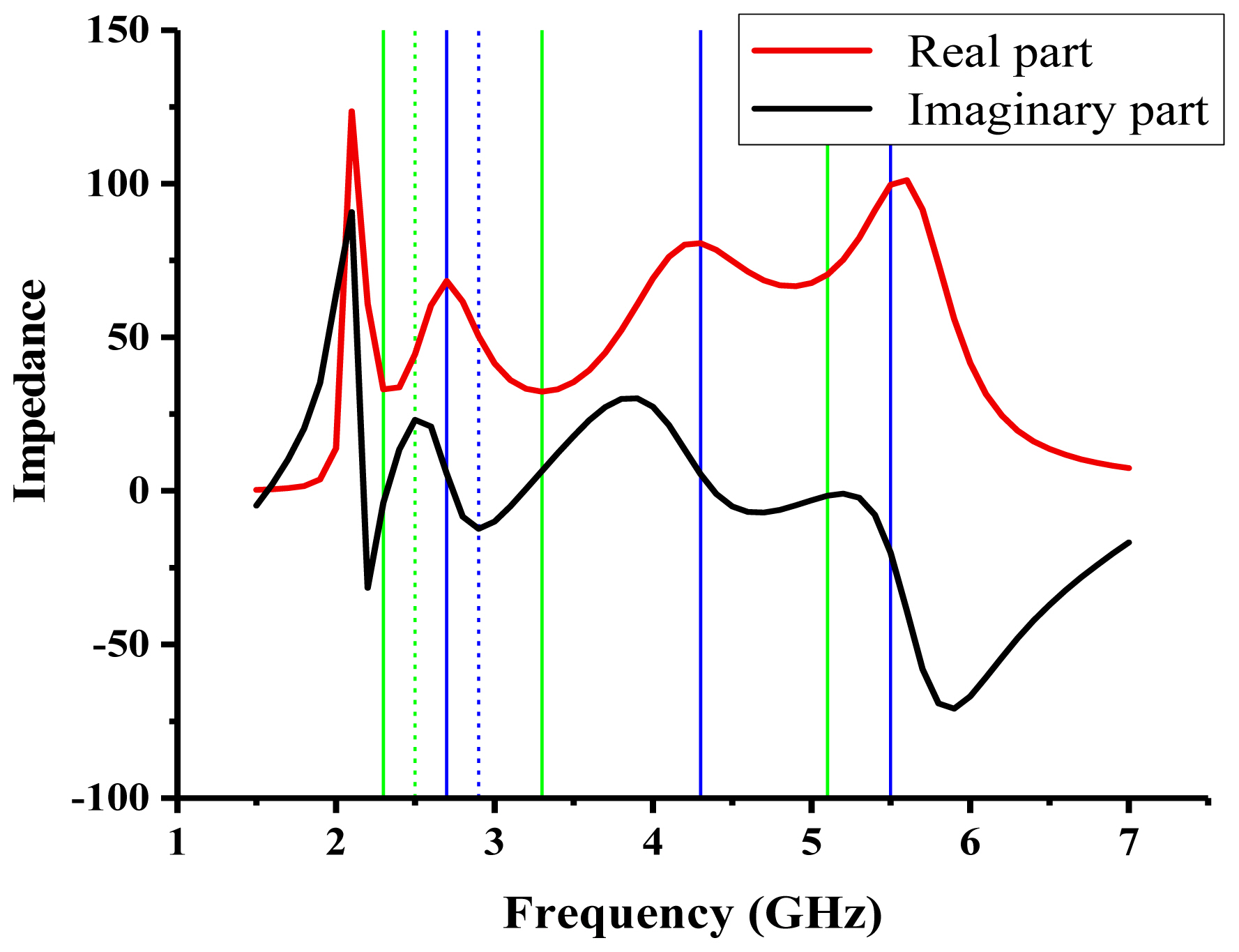
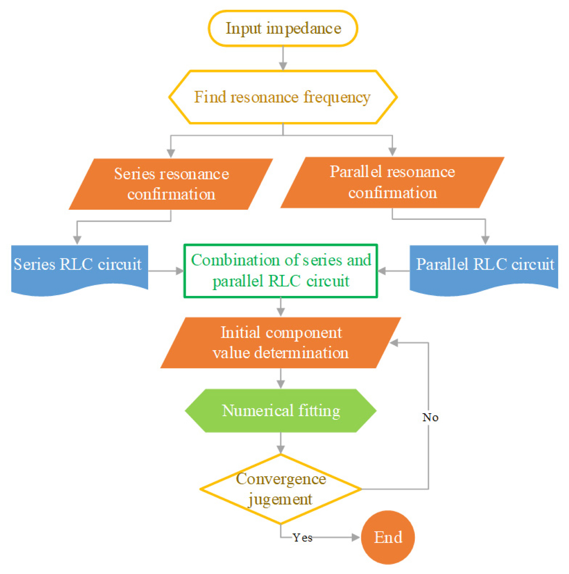
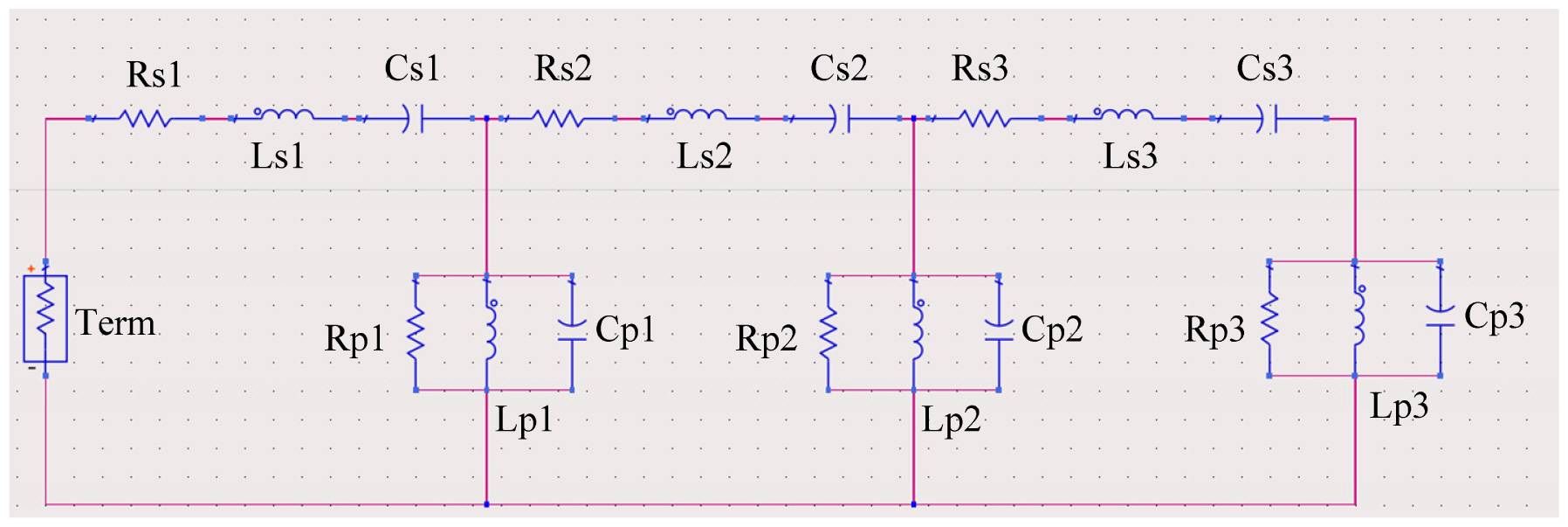
The first step of the extraction procedure involved simulating the input impedance of the basic ME dipole using the Ansys High Frequency Structural Simulator (HFSS), as plotted in Fig. 3. The operating band (2.2–5.5 GHz) comprised three series resonance points (marked by the solid green lines) and three parallel resonance points (marked by the solid blue lines). The series resonance points were located at 2.3 GHz, 3.3 GHz, and 5.1 GHz, with impedances of Zs1 = 33 Ω, Zs2 = 34 Ω, and Zs3 = 70 Ω. Meanwhile, the parallel resonance points were located at 2.7 GHz, 4.3 GHz, and 5.5 GHz, with impedances of Zp1 = 65 Ω, Zp2 = 80 Ω, and Zp3 = 100 Ω. Based on these series/parallel resonance points, the equivalent circuit was extracted, as depicted in the flow diagram in Fig. 4. First, the series resonance was corresponded to a series RLC circuit, as shown in Fig. 5(a). Second, the parallel resonance was corresponded to a parallel RLC circuit, as shown in Fig. 5(b). Effectively, three series circuits and three parallel circuits were obtained. Third, based on the order of the resonance frequency, the previously mentioned series resonance circuits and parallel resonance circuits were connected in sequence, as shown in Fig. 5(c), generating three series branches (Rs1/Ls1/Cs1, Rs2/Ls2/Cs2, and Rs3/Ls3/Cs3) and three parallel branches (Rp1/Lp1/Cp1, Rp2/Lp2/Cp2, and Rp3/Lp3/Cp3). To obtain the values of the components in Fig. 5(c), the initial values for all R/L/C had to be obtained in advance according to the impedance values at the corresponding resonant points. The detailed procedure to determine these initial values is discussed in the next section. Finally, a numerical fitting procedure was implemented based on the initial element values. After setting reasonable iterations and tolerance, the final equivalent circuit was realized.
3. Initial Value Determination
To obtain the final values of the components in Fig. 5(c), a fitting iteration process was implemented. This section demonstrates the method and the problems encountered in determining the initial values during the fitting iteration. For simplicity, only the first series resonance branch (Rs1, Ls1, and Cs1 in Fig. 5(c)) and the first parallel resonance branch (Rp1, Lp1, and Cp1 in Fig. 5(c)) are discussed in detail. Notably, the determination process for the other branches was the same as that for the first series and parallel branches.
To attain the first series resonance frequency fs1 (indicated by the first solid green line in Fig. 3), it was assumed that Rs1 is equal to the resistance (33 Ω) at the frequency point. The first extreme point in reactance after fs1 was termed ffs1, marked by the dashed green line in Fig. 3. The figure further shows that fs1 and ffs1 correspond to 2.3 GHz and 2.5 GHz, respectively. To obtain the Ls1 and Cs1 values for the first resonance subcircuit, two equations pertaining to Ls1 and Cs1 were formulated. The first equation was based on the assumption that the series resonance at frequency fs1 is caused by Ls1 and Cs1, while the second was based on the assumption that the total reactance value at ffs1 is the sum of the reactance of Ls1 and Cs1. Hence, the initial values for Ls1 and Cs1 were calculated using the following equations:
where ωs1 and ωfs1 are the angular frequencies of fs1 and ffs1, respectively. Furthermore, Xfs1 refers to the reactance at ffs1, which is equal to 23.3 Ω, as indicated in Fig. 3 by the intersection of the first dashed green line with the black line. By computing Eq. (1), the following values were acquired: Ls1 = 9.28 nH and Cs1 = 0.52 pF. Therefore, the initial element values for the first RLC series branch were calculated according to the first resonant frequency fs1 and the first extreme point after fs1.
Next, the initial component values for the first parallel branch were calculated according to the first parallel resonance frequency fp1 and the first reactance extreme point frequency ffp1 after fp1. Notably, ffp1 is denoted by the dashed blue line in Fig. 3. The results showed that fp1 = 2.7 GHz and ffp1 = 2.9 GHz, with the parallel branch composed of Rp1, Lp1, and Cp1. Similar to the calculations for the series resonance circuit, the initial Rp1 in the current estimation was equal to the resistance at fp1, as a result of which Rp1 = 65 Ω in this branch. Moreover, two additional equations were formulated to obtain the initial values of Lp1 and Cp1. In contrast to the series resonance circuit, the first equation in this case was a resonance equation that accounted for the resonance frequency fp1 at which a parallel resonance occurred. Meanwhile, the second equation was a susceptance equation, where the susceptance at ffp1 was assumed to be contributed by Lp1 and Cp1. Effectively, Eq. (2) were constructed to calculate Lp1 and Cp1, as follows:
where ωp1 and ωfp1 are the angular frequencies at fp1 and ffp1, respectively. Meanwhile, Bfp1 refers to the susceptance at ffp1, with a value equal to 0.0045 S. By computing Eq. (2)Lp1 = 1.73 nH and Cp1 = 2 pF were obtained.
The other series (Rs2/Ls2/Cs2 and Rs3/Ls3/Cs3) and parallel branches (Rp2/Lp2/Cp2 and Rp3/Lp3/Cp3) were calculated in the same way as described above. For brevity, the detailed deduction process is not presented here. After conducting a deduction process for each branch, the initial values of all components in Fig. 5(c) were obtained, as listed in Table 2.
4. Curve Fitting and Validation
Before curve fitting was performed, the input impedance expression for the circuit presented in Fig. 5(c) was estimated in advance. The impedance of the series branch and the admittance of the parallel branch were calculated using Eqs. (3) and (4), respectively, as follows:
Based on the above formulations, the total input impedance for the equivalent circuit depicted in Fig. 5(c) can be expressed as follows:
where Z2 can be calculated using the following equation:
To obtain a good fitting result, the objective function in the fitting algorithm was considered the difference between the input impedance at the antenna port and the equivalent circuit port, which can be expressed as:
where n refers to the total number of sample frequency points within the concerned frequency range and i indicates the i-th sample point. Therefore, delta_fun represents the algebraic sum of squares of the difference between the input impedances of the antenna and the circuit at all frequency points.
To obtain the values of the circuit components, this study adopted a numerical fitting technique using the MATLAB program in the least square sense. To achieve an accurate result, delta_fun was set to 0.05, while the maximum number of iterations was set to 8,000. The initial element values are listed in Table 2. Notably, the lower boundaries for R, L, and C were found to be zero, while the upper boundaries were 2,000 Ω, 500 nH, and 1,000 pF, respectively. The final element values were calculated by implementing the fitting process, the results of which are listed in Table 3. Based on the values in Table 3, a circuit model was built in the Advanced Design System for validation, as shown in Fig. 6. In this circuit, the source impedance was set at 50 Ω to maintain consistency with the characteristic impedance of the antenna port. The input impedance for the circuit illustrated in Fig. 6 is plotted in Fig. 7. Furthermore, the input impedance at the antenna port is depicted in Fig. 7 for comparison. It is obvious that the impedance curves for the equivalent circuit and the basic ME dipole antenna are in good agreement with each other. This agreement validates the reasonability and feasibility of the equivalent model and the robustness of the deduction procedure. Moreover, the proposed method is also applicable for extracting the equivalent circuit model for other types of antennas.
III. Conclusion
This paper numerically extracted an equivalent circuit model for a basic ME dipole. First, the structure of the basic ME dipole and its impedance were obtained. Second, the equivalent circuit form of the antenna was extracted based on series resonance and parallel resonance. Subsequently, the proposed circuit was composed of three series and three parallel resonance sub-circuits. Third, based on the resonance points and extreme points in the reactance, the initial values of the circuit components were calculated. The final component values were obtained by accurately implementing a numerical fitting. Notably, the extraction procedure involved both model establishment and numerical calculations. Finally, the equivalent circuit simulation and antenna EM simulation were observed to be in good agreement. As a result, it is established that the proposed equivalent circuit model offers good circuit representation for basic ME dipole antennas and exhibits great potential for use in antenna/circuit co-simulation.