A VAE consists of two sub-networks—an encoder, which typically reduces the dimensionality of input data, and a decoder, which reconstructs the input data from the reduced dimensional variables. An autoencoder (AE) [29] possesses this fundamental architecture, which enables the creation of a significantly reduced-dimensional hidden space between the bottleneck layers of its two sub-networks. The distance between samples in the latent space, constructed through identity mapping (perfectly reconstructing the original input), can capture semantic differences that remain concealed when using Euclidean distance in the original data domain. Notably, while an AE is usually utilized as a tool for feature extraction in classification problems or for dimensionality reduction in effective data compression, the VAE can also serve as a generative model by introducing stochastic variations to latent variables. The detailed structure of this function is illustrated in Fig. 1, where X, X̂, and z denote the input data, the reconstructed data of the input, and latent codes, respectively. The encoder of the first sub-network, denoted by E, is exploited to yield two intermediate variables, μ and σ², representing the mean and variance of a Gaussian distribution, respectively. Theoretically, latent codes z should be directly sampled using μ and σ² from the probability density function. However, in the given scenario, computing the derivatives becomes infeasible due to the randomness in the sampling step, which prevents the backpropagation of loss signals to previous layers. To address this problem, VAE employs a reparameterization trick by introducing a noise vector ɛ, randomly sampled from a normal distribution, and adding it to the variance σ². This concept can be briefly expressed as follows:

where the symbol ⊙ indicates the element-wise product, also known as the Hadamard product. The latent space, consisting of variable z, is shaped by the KL divergence scheme, as stated earlier. Notably, the variables sampled from the latent space can generate new examples (X̂), which are most likely to exist in the original data (X). Furthermore, the weights and biases of the learnable parameters in the neural network are optimized by means of a minimization strategy of the objective function, defined below:

where the total loss of L_VAE is a function pertaining to X of the input data, and the parameters of the two sub-networks, E and D, are denoted by φ and θ, respectively. The first term on the right-hand side represents the KL divergence, quantified as the difference between a posterior, fitted by optimizing φ in E, and a predefined prior. The second term serves as a metric to calculate the reconstruction error of X̂, generated by D_θ(z) in relation to the original data X. This metric can take the form of the mean squared error (MSE) or a binary cross-entropy (BCE), depending on whether the target data consist of real values or binary numbers.

The following subsection explores related research on this subject, especially focusing on how the standard VAE structure has been customized to address the inverse design of metasurfaces.

In [26, 30], the authors demonstrated the reliable reproducibility of the latent space achieved by VAE for new shapes of unit cells, justifying the applicability of their approaches in diverse scenarios. Notably, both works introduced an auxiliary network, termed the predictor, to tackle the one-to-many mapping problem occurring in an inverse design—one set of desired EM properties could be acquired by many different scatterer structures. The predictor is responsible for regularizing the latent variables learned through repetitive identity mapping of the source domain data, which might take the shape of either scatterers or EM properties. In other words, it is due to the effects of the predictor that the latent space can simultaneously represent the key features of two different data domains—scatterers and EM properties—thus, consequently being a vector in latent space that acts like an interpreter to translate the data of one domain into the data in the other domain. The architecture of the predictor can be realized using CNN or MLP.

Nonetheless, the noticeable points of difference between the two prior works are their choice of target and source domains for identity mapping in the VAE and for the regression of the predictor. Fang et al. [30] chose scatterer shapes as the datasets for conducting self-supervised learning in VAE, while EM properties were exploited as the target variables for the predictor model, and the latent variables determined by VAE were the input. The inverse model constructed by this training scheme presents various inverse design strategies working separately according to the meticulously devised criterion established for assessing the relevance of the outcomes. One of the most ideal scenarios for inverse design, assuming no failures, is as follows:

1. Prepare the desired EM properties,

2. Randomly draw initial values from the latent space,

3. Put the variable into the predictor network and obtain the predicted EM properties,

4. Compute the difference between the resulting EM properties and the desired ones by running a particle swarm optimization (PSO) algorithm,

5. Update the latent variables based on the optimization tactic of the PSO,

6. Repeat this process until a preset tolerance or an iteration number is reached.

In contrast to the strategy adopted in [30], the authors in [26] employed the EM properties for learning latent representation, while the pattern shapes of the metasurfaces were utilized as input for the predictor performing the regression to predict latent variables. Interestingly, latent variables learned by VAE serve as label data for the output of the predictor network. The learning rule for this setup can be expressed as follows:

where θ and K denote a set of parameters of the predictor model and the dimension of the vectors, respectively, while 〈 ·, ·〉 indicates the Euclidean distance of the two vectors. This framework estimates a new metasurface design for a set of desired EM properties by jointly operating the optimization process of the inverse problem and the forward design process, taking advantage of the latent presentation that concurrently retains the common nature of both domains involved.

The two exemplified frameworks have been proven to satisfy diverse inverse design requests, maintaining high accuracy in a wide range of applications. Moreover, they offer valuable insights into the successful adoption of the ML-based inverse design approach for the synthesis of metasurfaces. However, despite their remarkable achievements, the previous works are characterized by some arguable limitations, such as their need for vast amounts of training datasets, the usage of a dedicated external simulator, and the high complexity of operation involved in achieving satisfactory inverse design. To address these challenges, the current study focuses on developing a more streamlined end-to-end design approach that is both generally and readily applicable without the need for assistance from an external simulator or for considering complex options in the operational process.

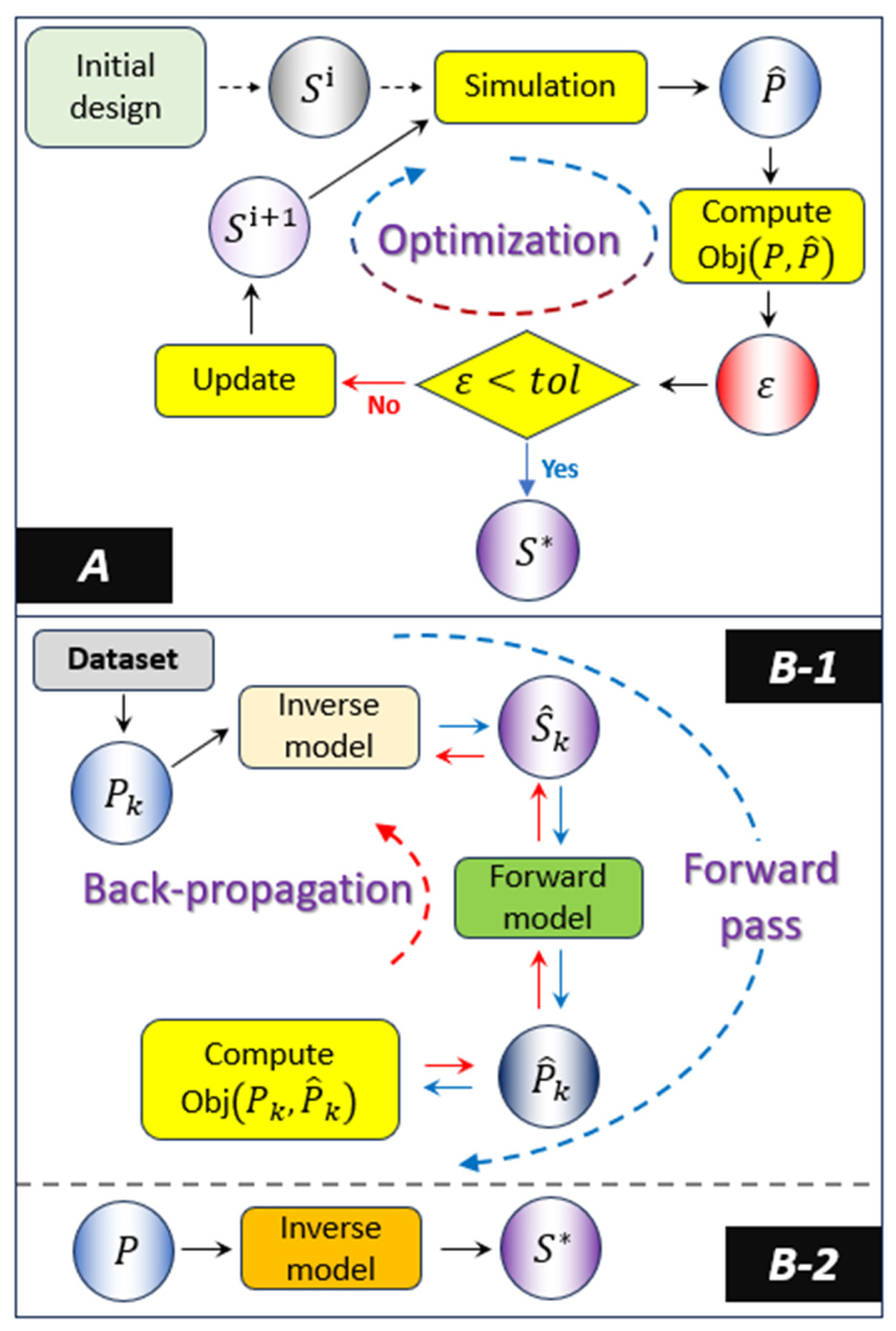
One of the significant advantages of ML-based inverse design methods relative to the conventional metasurface design process is that it does not need to conduct a brute force search by repeating full-wave simulations until the globally optimal solution is reached. However, to attain the benefits mentioned above in the design stage, data-driven approaches cost commensurate efforts—adequate data preparation, appropriate network design, and a robust validation process—in the model construction stage. The pros and cons of both concerned frameworks can be observed in Fig. 2, where block A visualizes the conventional design process and blocks B-1 and B-2 show the training phase and inference phase of an ML-based inverse design method, respectively. The symbols S and P represent the digital data corresponding to scatterer shapes and EM properties. It is evident that although the scheme in A does not require the preparation of a huge amount of datasets, it has to undergo many cycles of simulation at every design step. On the contrary, ML frameworks are able to markedly expedite the design process, as demonstrated in B-2, provided reliable neural networks are built in the B-1 learning phase. Nevertheless, the workflow of the inverse design depicted in B-2 may be considered ideal or extremely simplified, given the high degree-of-freedom exhibited by EMMS behavior, which varies with the design configuration. Moreover, the topology of the design space does not allow for the prediction of a unique solution. As a result, previous works were compelled to assume complex situations and set extra plans to address exceptional cases, due to which these frameworks require either an external simulator or the intervention of a human user. Inspired by the basic ideas enshrined in these existing works, the current study aims to develop a fully automated end-to-end ML-based inverse design method from scratch. To achieve this goal, additional useful information related to the geometry of EMMS, such as their types and dimension parameters, was employed. Furthermore, the architecture of the neural network was designed to reflect the roles pertaining to the additional information. Moreover, this work built separate latent spaces according to the types of EMMS to possibly predict equivalent EMMS shapes more precisely, owing to the reduction of ambiguity among the latent variables. The details are described in the next section.

The success of a data-driven approach is significantly influenced by the size of the training dataset and its relevance to the problem that users are facing, since weights in neural networks are fitted by interacting with features extracted from the dataset. To optimize the weights of a neural network, supervised-learning models utilize the loss signals yielded in the course of mapping the input data to the specified target data—a process referred to as function approximation. Therefore, to allow the function to faithfully relate two different domains, the pairs of input and output data should be informative and straightforward. Based on the above factors, the basic idea for synthesizing the training dataset used in this study was inspired by [26]. Furthermore, for the sake of accomplishing a more favorable function approximation, two additional data types—the class of the data and a set of numbers characterizing the geometry of the scatterer—were employed alongside the scatterer shapes and EM properties. These additional data not only provide increased information but can also be used to validate the results predicted by the proposed approach.

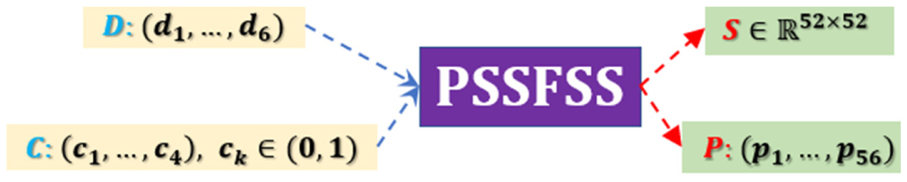
Meanwhile, the synthetic datasets were produced by PSS-FSS—a free and open-source code written in Julia programming language that was developed to design and simulate polarization selective surfaces (PSSs) and frequency selective surfaces (FSSs). Notably, to synthesize certain types of metasurfaces, PSSFSS requires several parameters to define the concerned shapes and materials. In this study, the additional data were used as the input arguments, based on which a comparison of the shapes of the scatterers acquired from the proposed method and from the PSSFSS can be conducted. Fig. 3 depicts the relationship among the four individual datasets, where C and D, corresponding to the additional dataset, are the 6-dimensional vectors specifying the geometry of shapes and categorical variables of one-hot encoding differentiating four classes of scatterer shapes, respectively. The denotations of S and P are the same as in the definition provided in Section II. In terms of data type, S is a 52×52 matrix consisting of elements with 1 representing a metallic area or 0 otherwise, while P is a vector having the length of 56. As stated earlier, while an inverse model aims to predict a corresponding S in terms of a desired P, the proposed approach seeks improvement in prediction accuracy by adding C and D to the canonical inverse process. Furthermore, the synthetic datasets were created by increasing each dimension of D(d₁,,,d₆) at uniform intervals with respect to four categories C(c₁,,,c₄) of surface shapes, i.e., Jerusalem cross (JC) patch, loaded cross (LC) patch, JC slot, and LC slot. Notably, the patches and slots were distinguished by identifying whether or not their shapes were composed of metallic material. The values for S and P obtained by the mean of PSSFSS are displayed in Fig. 4, where P considers only the reflection coefficients of EMMS.

In addition, the parameters for the substrate material on which the meta-atom was placed had the same specifications as all PSSFSS simulations, with permittivity, loss tangent, and thickness of 4.4, 0.02, and 1.5 mm, respectively. The total number of datasets generated was 2,000, which was further divided at a ratio of 4 to 1 for training and testing whether each type of scatterer was evenly distributed, respectively.

The framework proposed in this study follows a cascade structure in which the sub-networks—encoder (En), generator (Ge), and decoder (De)—are sequentially connected, as exhibited in Fig. 5. The most significant difference of this framework from the standard VAE illustrated in Fig. 1 is the generator (Ge) positioned between the latent variables z and the decoder (De), which plays a pivotal role in converting simple identity mapping from P to P’ into a joint learning neural network comprised of the inverse and forward models. Notably, during the training phase, the latent space learns the salient features shared by both the EM properties (P) and the design parameters of the metasurfaces (C and D). The learnt representation can continuously and infinitely span the feature space owing to the promising capability of VAE learning, although the current study used a discrete and small amount of training dataset, as stated in the previous subsection. Consequently, after terminating the training phase, z and the generator (Ge) were detached from the whole network and employed in an inverse design method. In this context, it should be noted that the generator (Ge^*) yielding S’ contributed only to reliably constructing the latent representation z. The output S’ was not utilized in the following networks, since C and D were adopted as parameters determining the shapes of the scatterers and not S. Fig. 3 justifies this strategy. In fact, it was expected that the loss signal measuring the discrepancy between the estimated S’ and the true S will have an effect on regulating the latent space because S possesses the equivalent visual information for the geometry defined by C and D. Similarly, the auxiliary output S’’ of the decoder (De) predicting P plays the same role of imposing a constraint. Regarding the input and output datasets of the decoder (De), interestingly, it was observed that the network (De) carried out identical functions as the simulator PSSFSS, as depicted in Figure 3. Moreover, this study intended to enhance the fidelity of the generator (Ge) by evaluating the outcomes of the inverse design during the training phase. To achieve this, the decoder (De) was devised to learn the functions of the PSSFSS producing the shapes S for scatterers with respect to the given C and D and then predict the EM properties P. Therefore, the updated rule of weights in the entire network can be expressed as follows:

where L_Total indicates the weighted sum of the losses calculated by all involved loss functions with respect to the total number of data U, Θ denotes all learnable weights in the entire network, is a generic term representing all kinds of training datasets, while α and β are the hyperparameters tuned by the user. Furthermore, in the second row of Eq. (4)L_KL is equal to the first term on the right-hand side in Eq. (2), while L_RE constitutes three loss functions of the network—Ge, Ge^*, and De—as follows:

where L_G* represents the cross-entropy loss obtained on computing the loss of estimates and the ground truth, while L_G and L_D are the loss functions obtained on computing both the cross-entropy and the mean squared. Notably, the types of loss functions were determined according to the data formats defined in the previous subsection.

As mentioned before, the dimension parameters of the datasets were synthesized based on four preset primitive patterns: JC (patch), JC (slot), LC (patch), and LC (slot). As a result, the frequency responses of each type of scatterer changed gradually, corresponding to alterations in the dimension parameters. However, the crucial characteristics, i.e., band pass, band stop, and bandwidth of the frequency response, were dominated by the type of primitive pattern. In this regard, identifying the type of scatterers prior to predicting their shapes based on a desired EM property could help enhance prediction accuracy. Along these lines, the authors of [21] proposed a classification for scatterer topologies by conducting principal component analysis (PCA) using a support vector machine (SVM), which represents a great achievement in the development of the inverse design method. Nonetheless, while this advanced approach carried out the classification using external modules, this study attempted to realize an end-to-end inverse design model by developing a neural network incorporating the classification process. The core idea was to utilize the separately distributed latent spaces illustrated in Fig. 6, constructed during the training phase, and operate them at four different KL divergence terms relative to each class, using the following equation:

where N implies that the Gaussian distribution is fitted by μ_l,c and σl,c2, which denote the mean and the variance, respectively, of a variable of l_th dimension among 16-dimensional variables corresponding to c_th class. Notably, these variables are learning μ_i and σi2, which refer to the pre-defined ideal values according to the types of scatterer shapes. Furthermore, symbolizes an indicator function whose output is 1 in the case of c = i, otherwise 0.

All simulations were conducted on a PC equipped with 32 GB RAM and an Intel Core i7-12700F CPU at 2.10 GHz. A total of 2,000 samples (500 samples per class across four classes) were synthesized, in accordance with the process described earlier. The samples were then divided into 1,600 training samples and 400 test samples, maintaining proportional representation across classes. The synthetic unit cells had a periodicity of 15 mm, and were postulated to activate at 10 GHz of the center frequency. In the training phase, the datasets were grouped into batches of 32 samples, using which the learnable parameters of the networks were updated for 1,000 epochs. Moreover, for evaluation, the metaatoms considered in the proposed inverse design method were simulated using PSSFSS, and the corresponding EM properties were estimated and then compared to the desired EM properties to establish the ground truth of the experiment. To measure prediction accuracy, this study employed the mean absolute error (MAE) of the computing differences between the two EM properties at each frequency point, which can be formulated as:

where P and P̂ are the desired and predicted EM properties, respectively, and i denotes one frequency point in 56 (N) points.

The reconstruction accuracy of the proposed network was investigated using the test datasets. Fig. 7 describes the network pipeline for implementing identity mapping to the EM properties. In this test, the latent space was formed only by the estimated mean values without variances, indicating that the inference should be a deterministic process. As stated earlier, since S’’ was treated as just a dummy variable in the inference phase, the performance in this test was evaluated by calculating the MAE between P and P’. In Fig. 8, the reconstructed data, represented by red dotted lines, are compared to the reflection coefficients of the true samples, plotted using blue lines. A visual assessment of the figure shows consistency between the recovered data and the input samples. Furthermore, Fig. 9 compares the means of the 400 samples at every frequency point of the true samples (blue line) and the estimated results (red line). The MAE calculated for all frequency points was estimated to be 0.57. From the numerical results and visual assessment in Figs. 8 and 9, it is observed that the identity mapping process for the EM properties, as depicted in Fig. 7, exhibits satisfactory reconstruction accuracy, implying that the individual sub-networks had faithfully learned the relationships among the input-output data pairs involved in learning whole networks. The following subsection examines the prediction accuracy of the inverse design for scatterer shapes.

To confirm whether the latent variables continuously and smoothly spanned the sample space (Z) during the training phase while using a small amount of discrete training datasets, samples (z_i’s) from the latent space were randomly drawn and fed into the PSSFSS and the decoder (De) through the generator (Ge), as shown in Fig. 10. The C’ and D’, estimated by the generator (Ge) using input z_i, fully contained the geometric information necessary for synthesizing a metasurface using PSSFSS. As mentioned earlier, PSSFSS predicts P after producing S using inputs C and D. Hence, if the result of MAE(P,P’) is meaningfully tiny, it indicates that the latent space Z is able to accurately represent the infinite EM properties created following the rule by which the training datasets are synthesized. More specifically, assuming that the desired EM property is P̂(= P), P’ decoded from both C’ and D’ must be comparable to P̂ due to the small amount of error of MAE, while P*=argminP′ MAE(P^,P′) can be estimated using trustworthy optimizers, such as PSO [31] or genetic algorithm [32]. As a result, C’ and D’, as estimated by (Ge), are equivalent to the shape of the meta-atom S inversely designed by the proposed framework, as illustrated in Fig. 5. Fig. 11(b) exhibits the shapes of the scatterers S’’ yielded by the proposed inverse design method, while Fig. 11(a) compares the EM properties (red dotted line) predicted by the PSSFSS simulator, using S’’ and the EM properties (blue line) produced by the variables in the latent spaces. In addition, the simulation results (green asterisk symbol *) of HFSS were simultaneously compared to substantiate the reliability of the simulation accuracy estimated by PSSFSS. A visual comparison of the red, green, and blue lines in Fig. 11(a), along with the MAE values on each graph, demonstrates the accuracy of the proposed inverse design method, both visually and numerically. While slight discrepancies exist in the results in the second row, the locations of peaks and troughs, as well as the trend of the transition, closely resemble the ground truth (the red and green lines).

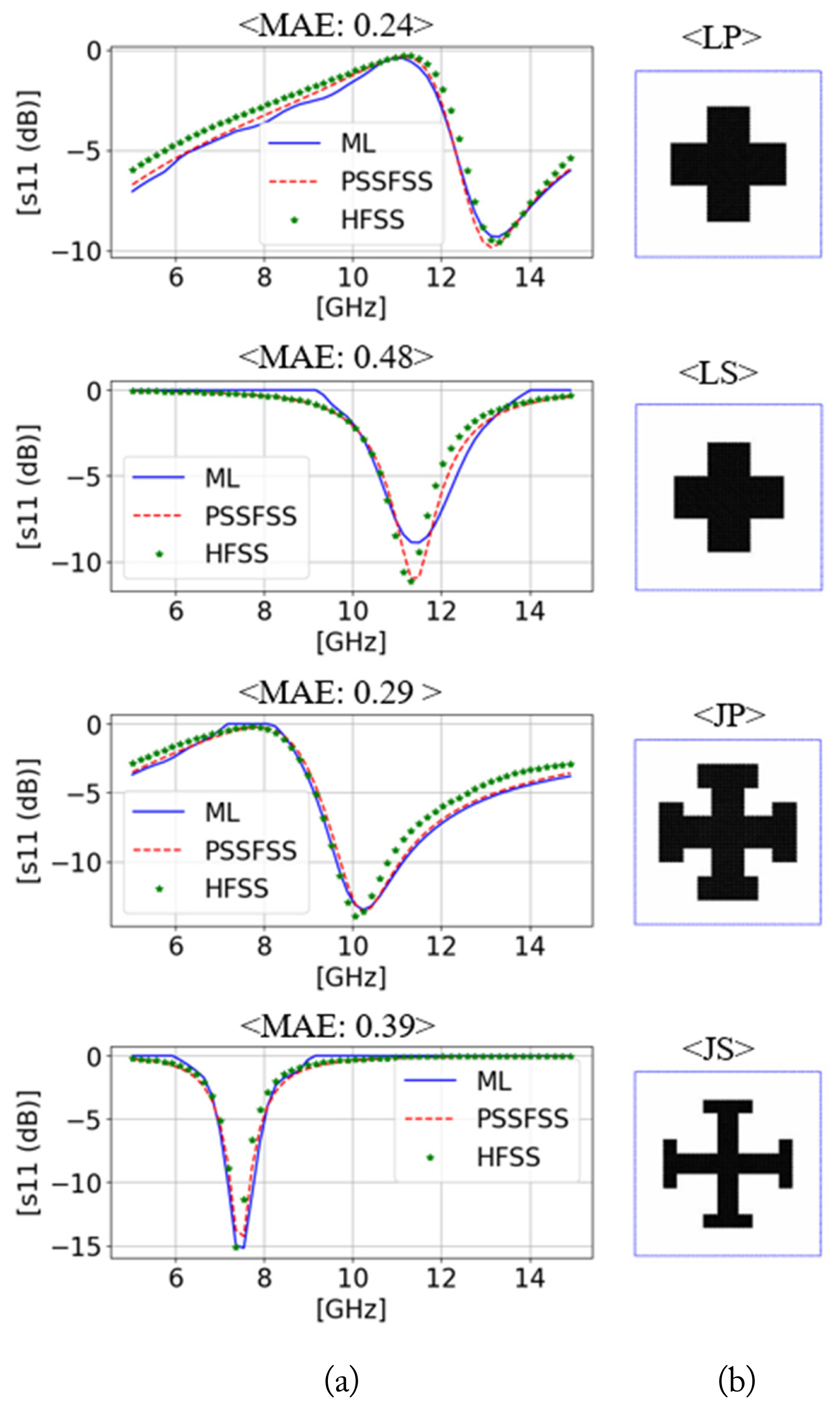
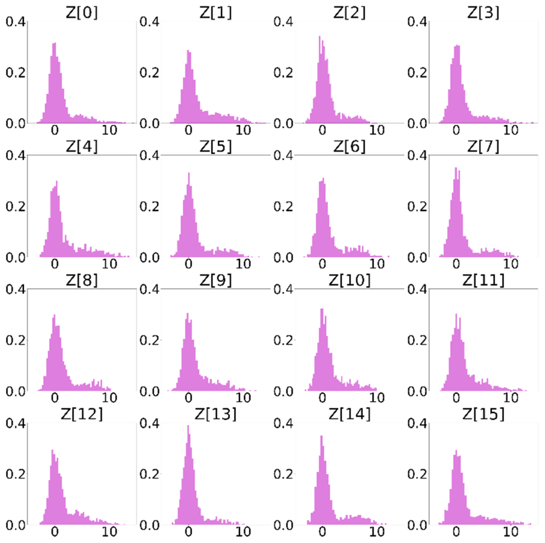
Finally, the impact of separately distributed latent spaces was investigated by comparing two cases—one with and one without the associated scheme. The test configurations were equal to the setup described in Sections IV-2 and IV-3. In the absence of the scheme, the reconstruction error (MAE) relative to the 400 test samples was 0.78, which was greater than the result acquired using separately distributed latent spaces by approximately 0.2. This implies that the model without the scheme demonstrated inferior estimation performance compared to the proposed method. In Fig. 12, the results obtained using the inverse design model with a single-distribution latent space are compared to those of PSSFSS and HFSS. The prediction error (MAE) of the variables sampled from the latent space is observed to be higher than the values computed with regard to the proposed approach in Fig. 11. Figs 13 and 14 clearly explain the consequences—the latent variables in Fig. 13 exhibit a single Gaussian distribution, while the variables in Fig. 14 show multiple peaks, similar to the Gaussian mixture model. Notably, this study intended to impose this characteristic of distribution on the latent space by taking advantage of Eq. (6) so that variables belonging to a certain class of scatterers could be sampled in terms of a unique mean value for the class. Using this strategy, variations in the EM properties for each class were clustered on a space independent from other classes, as illustrated in Fig. 6, making the process of searching relevant variables in the latent space more efficient and reliable. Nevertheless, in contrast to the expected outcome, the distributions exhibited in Fig. 14 do not characterize the perfect four Gaussian mixture model, with the distribution of Z[12] seemingly failing to learn the mixture distribution As mentioned before, only 2,000 samples were analyzed in this study, which were again split into 500 samples for each class. It is evident that the quantity of datasets used is inadequate for fully learning the intended distribution during the training phase. However, increasing the number of training datasets is likely to address this problem. The following section highlights the significance and contribution of the current study while also noting the limitations of the current work and directions for future research.