


I. Introduction
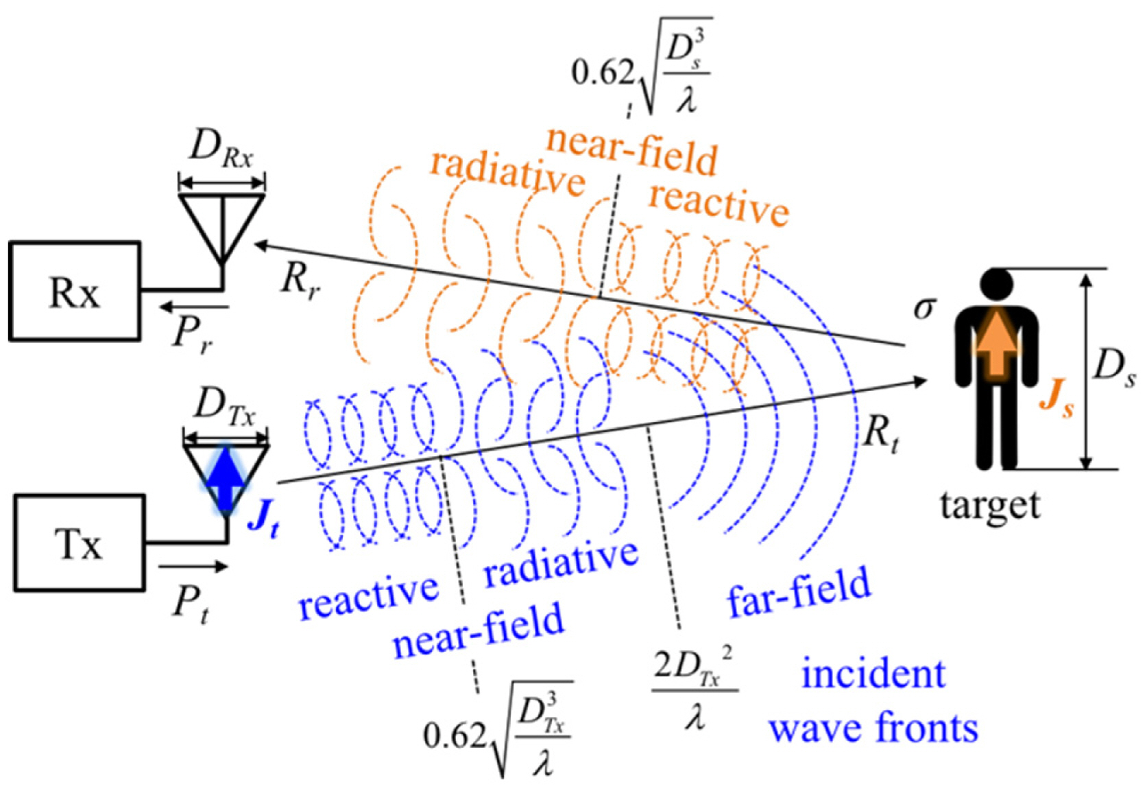
The automotive radar, generally categorized as long-range, mid-range, and short-range radars (LRR, MRR, and SRR, respectively), are an indispensable part of autonomous cars. For a decade, LRRs and SRRs have been developed to operate at 76–77 GHz [1] and 77–81 GHz [2, 3], respectively. Specifically, SRRs are usually employed to detect short-range targets, such as humans, to avoid collisions or crashes. Furthermore, as shown in Fig. 1, they typically have a quasi-monostatic structure.
The design phase of a radar system first involves conducting a link budget analysis. In this context, many researchers have continued to use the following classic radar equation for the development of an SRR [4, 5]:
where Pt and Pr denote the transmitted and received powers, respectively, and Gt and Gr refer to the gain of the transmitting and receiving antennas, respectively. Furthermore, σ is the radar cross section (RCS) of a target in m2 and Aer indicates the effective area of the receiving antenna, which usually becomes Grλ2/(4π). In addition, λ is the transmitted wavelength, R is the distance between the radar and the target, and Rt ≒ Rr ≡R for the quasi-monostatic radar. The most significant feature of (1) is that the received power decreases as the fourth power of R. However, this equation is valid only under conditions where the receiving antenna is situated far from the target and the target is also located at a substantial distance from the transmitting antenna.
Similarly, in the field of wireless communication, since users or scatterers are usually located in the near-field region of the reconfigurable intelligent surface (RIS) due to its large physical dimension, research on beam focusing, localization, and channel model of the RIS has received substantial attention [6, 7].
Through its measurement and simulation results, this paper highlights that the above-mentioned conditions are not satisfied when an SRR detects humans or cars at a short distance. Furthermore, it proposes a near-field radar equation by drawing on near-field characteristics and validates it using the measured and simulation results
II. Effect of Large Target
It is well known that in circumstances where the maximum dimension D of an antenna is larger than its wavelength, the regions of the electromagnetic field around the antenna can be divided into the reactive near-field, radiative near-field (Fresnel), and far-field (Fraunhofer) regions. The most well-known boundaries between these three regions are 0.62(D3/λ)0.5 and 2D2/λ [8]. Additionally, the D2/4λ and 0.6D2/λ criteria have also been frequently cited in estimating the extent of near-field and transition (Fresnel) regions [9].
In conventional numerical techniques, such as physical optics and method of moment, the first step involves obtaining the induced current on a scatterer, based on which the scattered field is calculated, from the incident field. This concept is commonly considered when calculating scattered fields from a target [10] and designing reflector antennas [11].
Fig. 1 depicts the application of this relationship between the induced current and the scattered field on a general radar target. If the electromagnetic wave generated by current Jt on the transmitting antenna results in forward propagation of the target located in the far-field region, it can be considered that a uniform plane wave is incident on the target. This incident wave induces current Js on the target, after which the induced current generates a scattered field. These sequences can also be calculated using the surface equivalence principle and radiation integrals [8]. In this context, it should be noted that the target in this example acts as an antenna with dimension Ds due to the induced current Js. Therefore, even when the target is located in the far-field region of the transmitting antenna, the receiving antenna may not be within the far field of the target due to the target’s dimensions.
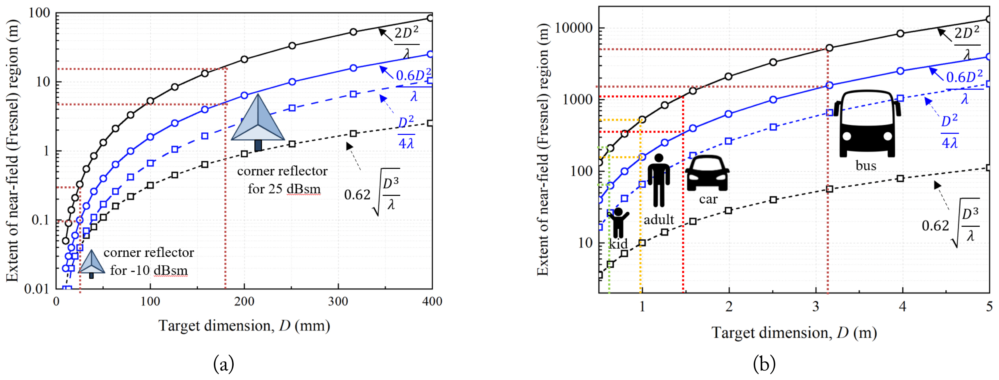
Fig. 2 presents the two boundaries in the near and far scattered fields from a target with respect to the target dimension. For automotive radar tests, corner reflectors are generally used as substitutes for real targets, such as humans and other vehicles. This study used corner reflectors of dimensions 25 mm and 180 mm, characterized by RCS values of about −10 and 25 dBsm at 79 GHz, respectively, representing the values for a child and a bus. Since corner reflectors exhibit high RCS for small sizes, the far-field distance was observed to be only several meters. For the 25 dBsm reflectors, a distance of only 5–18 m was required for the far-field region. Therefore, it can be assumed that the receiving antenna is located in the far-field region. However, real targets that need to be detected by SRRs are usually much larger than corner reflectors, ranging from a 1- m-tall child to a 3.5-m-high bus.
The scattered field from a human body is predominantly determined by the upper body rather than the legs. As a result, the effective target dimensions of a 1-m-tall child and a 1.7-m-tall adult might be smaller than their actual heights. Similarly, the effective target dimensions of a 1.5-m-high car and a 3.5-m-high bus need to account for gaps between the road and the vehicle floor, rounded bodywork, and windshields. As shown in Fig. 2(b), for a receiving antenna to be located in the far-field region of a 1-m-tall child, it should be situated more than 50 m away from the child. In this context, a maximum detectable range (MDR) of 30 m for SRRs would ensure that the receiving antenna is within the reactive near-field region of the real targets. In other words, the scattered field from real targets cannot be incident on the receiving antenna in a plane wave. This means that (1) cannot estimate the exact received power in such situations, leading to an inaccurate link budget analysis for short-range targets.
This study also confirmed the effects of a large target through electromagnetic simulations using CST Microwave Studio’s Integral Equation Solver. For this purpose, a simple square perfect electric conductor (PEC) plate was considered the target in the far-field region of the transmitting antenna with an operating frequency of 79 GHz. It was assumed that a plane wave is incident on the target, as shown in Fig. 3(a). By varying the target size W based on a fixed simulation dimension, the electric field distribution was calculated with respect to the distance from the target. Fig. 3(b) and 3(c) show the total field (i.e., both the incident and the scattered fields) covered by PEC rectangular plates with widths of 100 mm and 10 mm, respectively. In this context, it should be noted that the total field patterns of the two cases are entirely different. As expected, the electric field generated by the larger scatterer exhibits fluctuating characteristics in the reactive near-field region, as well as a characteristic decrease after a slight increase in the radiative near-field region. This further indicates that the entire analysis region is in the near-field region. In contrast, the small scatterer exhibited a very short near-field region.
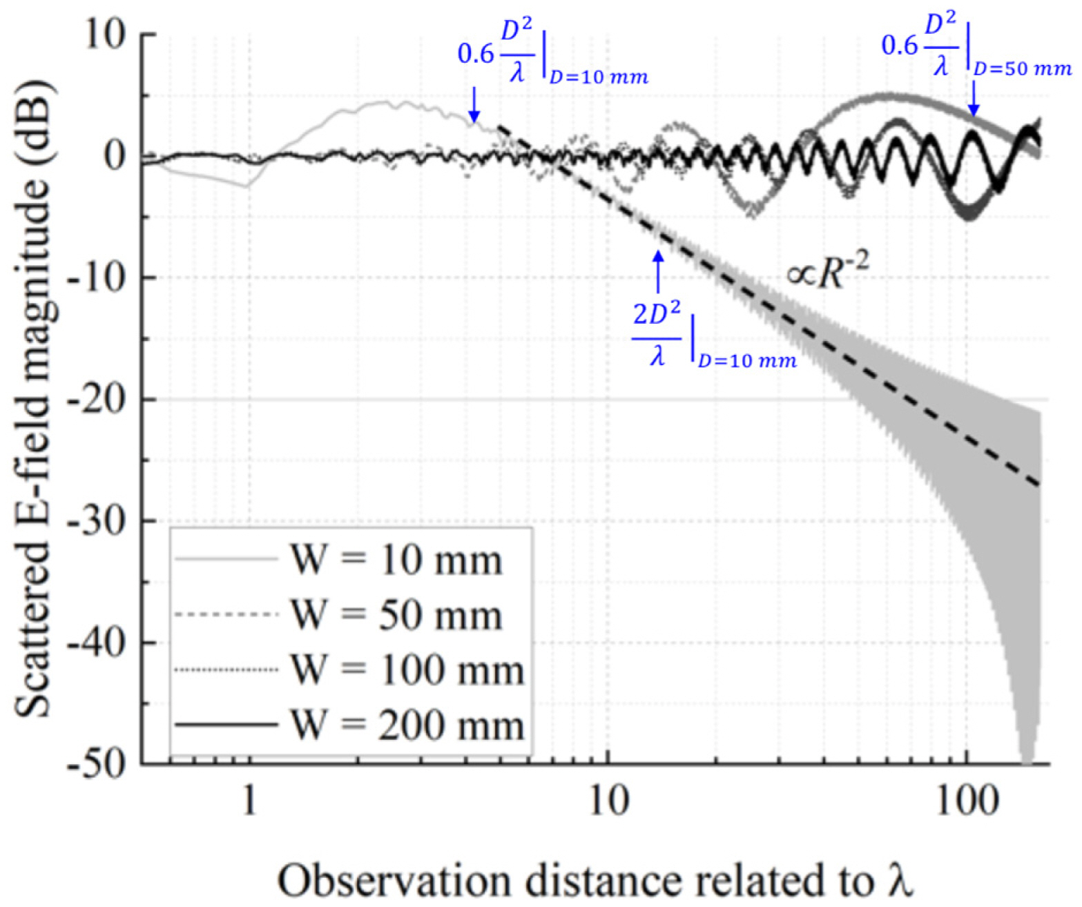
Fig. 4 presents the scattered fields obtained by removing the incident field from the total field along the central perpendicular axis of the scatterer for several rectangular scatterers. Since the analysis regions for rectangular plates of W = 50, 100, and 200 mm are in their near-field regions, their scattered fields fluctuate around 0 dB and remain fairly constant at various distances from the scatterer. Similar results have been reported in [12]. In contrast, the scattered field created by the small scatterer with W = 10 mm decreases proportionally with the inverse-square of distance (1/R2) from around five wavelengths after fluctuation, which is closer to 0.6D2/λ than 2D2/λ.
This study also verified the effects of a large target on the scattered field through conducting experiments in which a selected radar module had to detect an adult with regard to variations in radar module height, as shown in Fig. 5. Since this radar module involved an SRR and was developed to be mounted on large vehicles, such as buses and heavy vehicles, its height was modified rather than the range of the target. Furthermore, in this radar module, the receiving and transmitting antennas possessed the same structure and gain, Gt(θ)=Gr(θ), while a constant false alarm was used to detect the target against background noise and clutter. Table 1 presents the measured MDR results obtained for several radar module heights.
Since the changes in the height of the radar were smaller compared to the distance between the radar and a human target, the constant RCS and distance R′ were regarded as σ and MDR R, respectively. Meanwhile, the angle of direction to the target registered a maximum 4° difference depending on the radar height. Since automotive radars generally possess a narrow beam width at an elevation angle to achieve high antenna gain, the detectable range changes in relation to the radar module height can primarily be attributed to antenna gain in the direction of the target.
where E is the far-field strength in V/m and η represents the wave impedance. Furthermore, if the classic radar equation is effective in this situation, the received power scattered from the target located at the MDR can be formulated using (1) and (2), as follows:
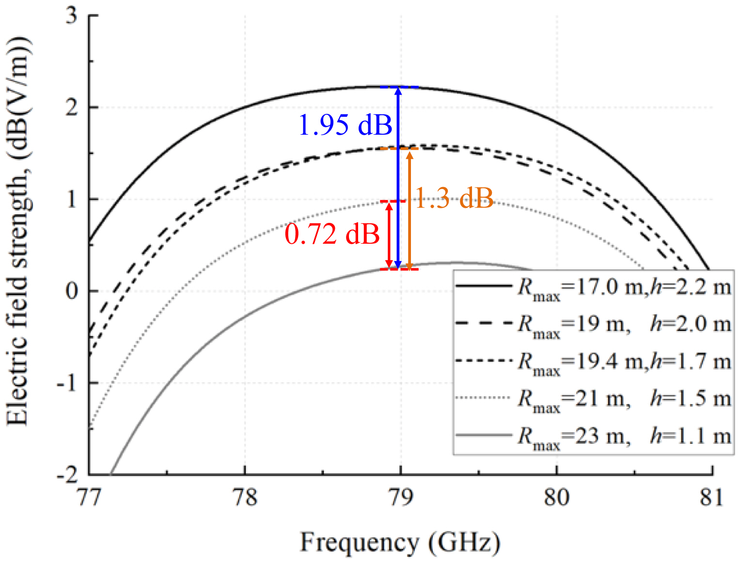
which indicates the smallest received power above the detection threshold relative to the noise and clutter signal, referred to as the minimum detectable signal (MDS) [14]. The MDS of (3) generally remains unchanged unless there are significant fluctuations in the noise or clutter signal. If the classic radar equation in (3) is valid for a large target, as in the case of this experiment, the electric field strength |E(Rmax,θ)| must be identical at all MDRs, since Pt and σ are also constant.
To obtain |E(Rmax,θ)| at the MDRs, only the target was removed from the setup presented in the actual experiment, after which the electric field from the radar antenna was simulated using the CST Microwave Studio. Fig. 6 illustrates the simulated electric field strength at the MDRs listed in Table 1. At the center frequency of 79 GHz, the electric field strength presents different values for the MDRs. This indicates that the classic radar equation is unsuitable for a large target. Therefore, a new radar equation is required for situations in which the receiving antenna is located in the near-field region of the target.
III. Near-Field Radar Equation
1. Formulation
To formulate a new radar equation for the near-field region, propagation characteristics in the region had to be formulated. To simplify this problem, a rectangular plate was considered the target, as shown in Fig. 7(a). According to Love’s equivalence principle, an aperture of width Tw and height Th in an infinite ground plane and a plate of width Tw and height Th in free space are complementary structures, as shown in Fig. 7(b). Therefore, the scattered field can be obtained from field E0 on the aperture instead of the current density Js on the metal plate.
Based on the assumption that the observation point is located farther from the target’s dimensions, (x − x′)2 + (z − z′)2 << y2. Therefore, the distance from the origin of the aperture can be approximated as follows:
Based on the assumption in (4), the field strength in the near-field region can be obtained from the Fresnel diffraction formula [15] as follows:
where field E0(x′,z′) in the aperture represents a part of the incident field from the transmitter. Therefore, from (2), E0(x′,z′) can be expressed as:
where Γ is the reflection coefficient of the target, which is dependent on the incident and scattered angles, as well as the material characteristics of the target.
Furthermore, if field E0(x′,z′) is uniformly distributed in the aperture, it becomes a constant value of E0. In such a case, the scattered field can be formulated as follows:
Subsequently, using the complex Fresnel integral F(z), the field can be attained from the following equation:
where the complex Fresnel integral F(z) and parameter q can be defined as:
Notably, the Fresnel integral in (9) can be calculated using the approximation equations noted in Appendix A.
Effectively, the electric field at the height of the radar at distance R away from the aperture can be presented as follows:
In addition, by multiplying the scattered power and the receiving antenna aperture area, the received power can be estimated as follows:
where qR = (2/λR)0.5. In this context, it should be noted that the derived near-field radar equation in (13) would be valid only when the distance between the observation point and the target is greater than the target dimension, i.e., in the Fresnel region, due to (4).
Fig. 8 depicts the received power, calculated using (13), with respect to the distance between the radar and the target. This calculation assumed that the receiving module is placed at distance R from the plate at a height of 1.72 m, bearing a width of 0.55 m. As depicted in Fig. 8, the received power declines up to approximately 70 m, after which the square of distance begins to decrease stably until the fourth of the distance reaches about 400 m, which is closer to 0.6D2/λ than 2D2/λ. Notably, the results obtained for the near-field region contrast sharply with those of the classic radar equation in the far-field region. In addition, the near-field radar equation in (14) can be applied to both far-field and near-field regions. Notably, if the receiving antenna is located in the far-field region of the target, the equation in (14) will become the classic radar equation presented in (1). This transformation process is detailed in Appendix B.
2. Verification with Simulated and Experimental Data
As mentioned earlier, considering the same false alarm rate and transmitted power, the received power at the MDR should be as constant as the MDS. Therefore, to verify the proposed near-field radar equation in (13), the received power at some MDRs was calculated to confirm whether they had identical received power.
The received power was calculated by incorporating the measurement results in Table 1 and the simulated results in Fig. 6 into the near-field radar equation in (13). However, since the transmitted power and reflection coefficient data of a human were not available, the received power ratio was calculated rather than the absolute received power. Notably, if the proposed near-field radar equation is valid, the received power ratio would be either 1.0 or 0 dB. In this context, the ratio of the received power in Rmax1 and Rmax2 can be expressed as follow:
(15)
where the first term on the right side of the equation—the electric field strength—is obtained from the simulated results presented in Fig. 6, while the second term is calculated using the approximation solution in (A1)–(A7) for each radar height and MDR. These results are summarized in Table 2, where the RCS component and received power component are expressed as |E(Rmax,θ)|2 and |E(Rmax1,θ)|2·|F(qRmax,Tw/2)|2 the right side of the equation in (15), respectively.
The fifth row in Table 2 notes the ratio of the received power at the radar height to that at 1.5-m height in the near-field, calculated using (15). Since the power level fluctuates instead of decreasing smoothly as the distance increases in the near-field region, and because the variability caused by the inaccurate target height is large, the received powers are not observed to be identical to each other. However, they showed similar values, with an error of less than 0.3 dB. This indicates that the proposed near-field radar equation is in good agreement with the measured MDRs for several SRR module heights.
Furthermore, assuming that the receiving antenna is located far from the target, the far-field RCS of the target was obtained from (B7). The far-field values corresponding to the RCS and the received power components in the near field are listed in rows 6–8 of Table 2. The results show that although the received power and the MDR should be almost the same, a maximum error of about 3 dB is observed. In addition, the fourth power relation between the received power and the target range is the result of having an excessively larger received power component value than the actual value in the near field. This highlights that existing far-field radar equations pertaining to the near field are inaccurate.
IV. Conclusion
This study proposed a novel near-field radar equation that is valid in the Fresnel region based on the Fresnel diffraction formula. The major feature of this equation is that the dependency of the distance between the radar and its targets is not considered as the negative fourth power of the distance, but as its negative square. Notably, various MDRs could be explained by the application of the proposed radar equation to the measurement results. However, to achieve a more accurate analysis of automotive radars, such as SRRs, further research on near-field receiving antenna gain and RCS is necessary.