


I. Introduction
Electromagnetic radiation sources (EMRSs) usually cause interference with electronic devices at the same frequency. In the context of electromagnetic environment monitoring systems, it is crucial to separate electromagnetic radiation signals of the same frequency to accurately detect and identify electromagnetic interference sources [1]. Blind source separation (BSS) is a technique that can extract source signals from mixed signals captured by multiple sensors, and this has been widely applied in speech processing [2], biomedical signal processing [3], image processing [4], fault diagnosis [5], and many other fields.
Traditionally, BSS can be assigned to overdetermined cases (M > P), determined cases (M = P), and underdetermined cases (M < P). Here, P is the number of sources, and M is the number of sensors. Currently, BSS methods can be broadly classified into three main categories, which are based on independent component analysis (ICA) [6], nonnegative matrix factorization (NMF) [7], and sparse component analysis (SCA) [8], respectively. The algebraic Jacobi method is used for the eigenvalue decomposition of FastICA [9], which improves the computation speed. However, it is not applicable to underdetermined cases. Leplat et al. [10] proposed a new NMF model based on the minimization of β-divergences and a penalty term for blind audio source separation. Ince and Dobigeon [11] introduced a residual weighting mechanism into the NMF for hyperspectral separation. However, NMF is very sensitive to noise and initialization, and its use for underdetermined BSS requires prior knowledge of various sources. The SCA-based method is the most popular underdetermined BSS method nowadays, which consists of three stages. The first stage is mixed signal sparsity, commonly transforming the observed signals into the time-frequency domain [12, 13] to ensure that the source signals are sparse enough, which is not suitable for multiple radiation sources of the same frequency. The second stage is the mixing matrix estimation, where the most common method is clustering, in which the mixing matrix estimation is transformed into an eigenvector clustering problem [14–16]. The unknown number and initial values of clusters make it very difficult to estimate the mixing matrix. The third stage is source recovery, which reconstructs the most likely version of the true sources by building an optimization model. For example, l1-norm penalized least squares is used to derive the sparsity-based non-linear signal separation model in [17]. Mixing matrix estimation and source recovery in underdetermined cases are still tricky problems. Moreover, the number and direction-of-arrival (DoA) of sources are crucial to mixing matrix estimation.
Recently, due to the increased availability of computing resources and the advancements in deep learning, the methods for estimating the number of sources and DoA have seen a shift toward the use of fully connected (FC) networks [18] and convolutional neural networks (CNNs). However, networks composed entirely of FC layers require more optimization parameters and computational resources. DoA estimation networks based on CNN discretize the angular domain into grids and deduce the DoA by determining the peak values in the respective spectrum [19, 20]. A drawback of this approach is that a minimum direction difference between the two sources and the number of sources must be predefined so that each grid is associated with only one possible source.
This paper discusses a method for separating EMRSs of the same frequency, even when the number of sources is unknown. The major contributions are three-fold.
1) A new separation method for EMRSs is proposed, which includes five steps: spatial spectrum estimation, EMRS number and DoA estimation, mixed matrix estimation, separation matrix estimation, and source signal recovery.
2) A pseudospatial spectrum estimation network (PSSNet) with a symmetrical CNN structure and a fusion layer is proposed for the first time in this field of application to estimate the number and DoA of EMRSs and the mixing matrix.
3) A new loss function is proposed as the optimization criterion to estimate the separation matrix. The separation matrix is estimated by optimizing network parameters for the first time.
The following mathematical notations are used throughout the paper: lower-case letters refer to variables, upper-case letters to scalars, bold lower-case letters to vectors, and bold upper-case letters to matrices. Transposition and Hermitian transposition of a vector and matrix are, respectively, denoted by [ ]T and [ ]H. Estimators are denoted by adding a hat onto the estimated variable.
j = - 1
II. Procedure of the Proposed Separation Method for Electromagnetic Radiation Sources
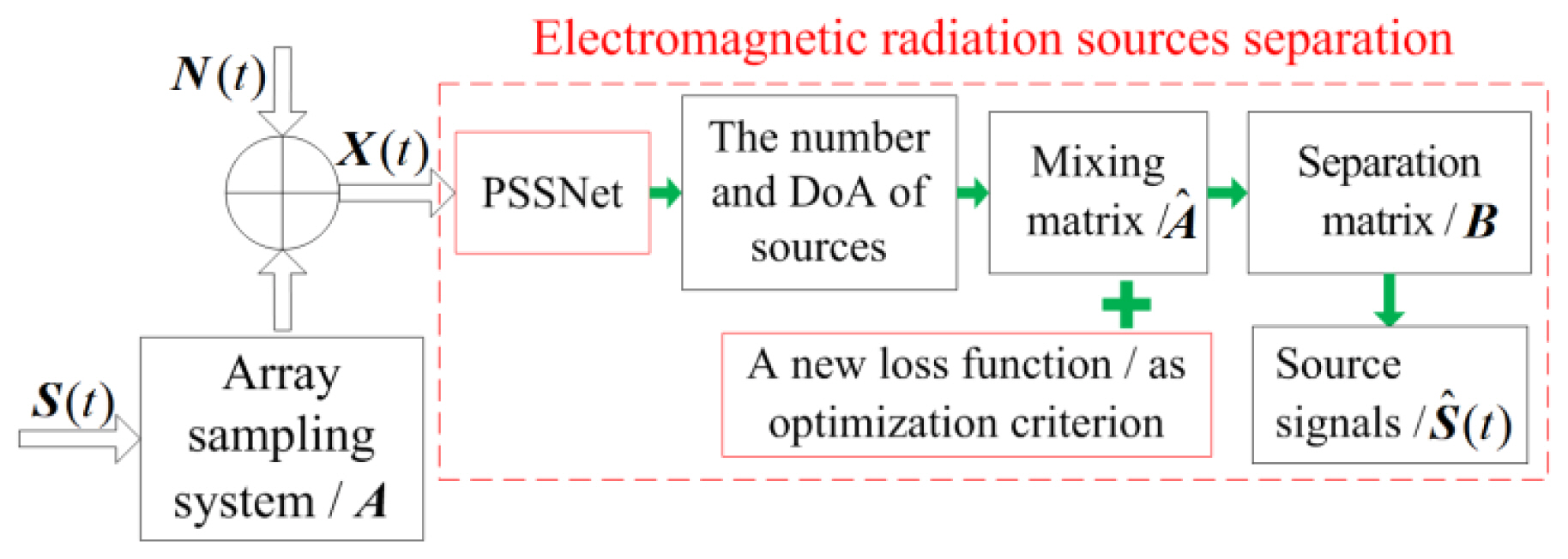
Inspired by the three stages of the BSS method based on SCA, an EMRS separation method is proposed, the flow chart of which is depicted in Fig. 1. In detail, it consists of five steps: spatial spectrum estimation, estimation of the number and DoA of EMRSs, mixing matrix estimation, separation matrix estimation, and source signal recovery.
X(t) is the observed signal obtained through the array sampling system, which is
where X(t) = [x1(t), x2(t), ···, xM(t)]T is the radiation signal observed by M arrays at time t, S(t) = [S1(t), S2(t), ···, SP(t)]T is the source signals matrix of P EMRSs, A denotes M × P dimension mixing matrix, and N(t) = [n1(t), n2(t), ···, nM(t)]T represents additive white Gaussian noise.
Array sampling systems usually observe electromagnetic radiation signals in a given environment through a uniform circular array (UCA) antenna. With the UCA center as the reference point, then the delay of the p-th source signal received by the m-th array and the reference point can be expressed as
where θp denotes DoA of the p-th source signal, R is the radius of the UCA, and C is the propagation speed of the radiation signal in space. The M × P dimensional mixing matrix is composed of P steering vectors, which is
The steering vector of the p-th source signal is shown in Eq. (4), which is located at the top of the page. Let  be the estimation of the mixing matrix and B be the P × M dimensional separation matrix. In the case of ignoring noise, the recovered source signal Ŝ(t) can be written as
Obviously, the source signal can be well recovered when BÂ = I, where I denotes the unit matrix. In the determined case, Â is a non-singular matrix, and B is the inverse of Â. However, it is still a great challenge to estimate A and B in overdetermined and underdetermined cases.
Therefore, the PSSNet based on CNN is built to get  by estimating the number and DoA of sources first. Afterward, A new loss function is proposed as the optimization criterion to estimate B.
III. PSSNet and Mixing Matrix Estimation
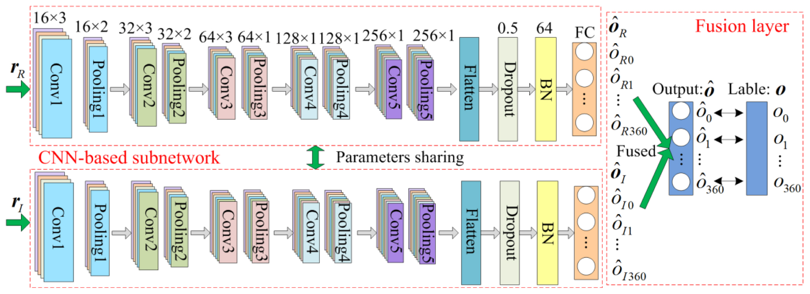
Utilizing neural networks to directly estimate the number and DoA of sources, one needs to define the maximum number of sources. In this section, the new PSSNet is constructed to generate a sharp PSS of sources. Then, the accurate source number and DoA are obtained according to the pseudospatial spectrum, and the mixed matrix is calculated according to Eqs. (3) and (4). Fig. 2 shows the architecture of PSSNet, which includes data preprocessing, two identical CNN-based subnetworks, and a fusion layer.
First, the observed signal is preprocessed. The observed signals from the array sampling system are in matrix form; its covariance matrix is a symmetrical complex matrix, so only the upper right corner elements are taken as the input of PSSNet for reducing the calculation, which has been shown to be a good pre-processing step for the complex observed signals in DoA estimation [21, 22]. The complex vector requires a complex deep network to implement the mapping. Therefore, the real and imaginary parts of the input vector are separated as rR and rI and are input to two subnetworks, respectively.
Second, based on the advantages of “local connection” and “parameter sharing” of CNN [23], the CNN-based subnetwork is constructed to quickly map the real and imaginary parts of the input vector to the spatial probability, which consists of five convolutional (Conv) layers with rectifier linear units (ReLUs), one flatten layer, one dropout layer, one batch normalization (BN) layer, and one FC layer. One max pooling is used after each Conv layer to select the local maximum of the vector as a statistic to highlight the amplitude characteristics of the radiation source. The FC layer maps the previously obtained feature vector to a 361-dimensional vector, representing the probability of source signals in directions 0°, 1°, ..., 360°. The output of two subnet-works are denoted as ôR = [ôR0, ôR1, ···, ôR360] and ôI = [ôI0, ôI1, ···, ôI360].
Third, the fusion layer is proposed to fuse the outputs of two subnetworks into one vector. The output of PSSNet is expected to be a “needle-like” PSS; i.e., the source signal has a probability of 1 in its direction, otherwise 0. The output labels for both subnetworks are the same, so the smaller one close to 0 or the larger one close to 1 in the output of two subnetworks are selected in the fusion layer. Let o = [o0, o1, ···, o360] be the output label of PSSNet and the two subnetworks, then the i-th output value of PSSNet is
where oi ∈ [0,1] is the i-th output label of the two subnetworks. Consequently, the estimation of PSS is ô = [ô0, ô1, ···, ô360].
Fourth, the estimation of PSS is formulated as a multilabel multiclassification problem, which includes 361 classes. Therefore, the loss function of PSSNet can be expressed as a binary cross-entropy loss [24]. Specifically,
where Q is the number of samples.
o i q ∈ [ 0 , 1 ] o ^ i q ∈ [ 0 , 1 ]
Finally, the DoA and number of EMRSs are estimated, and the mixed matrix is calculated. The “needle-like” PSS obtained by PSSNet is the probability distribution of radiation sources in space, which is sparse enough to easily obtain the number and DoAs of radiation sources. In theory, the DoAs of EMRSs are indices of 1 in the PSS estimation vector, and the number of EMRSs is the number of 1 in the PSS estimation vector. Unfortunately, the loss function is difficult to converge to 0, and it can only be infinitely close to 0. Again, ôi is very close to 1, but is not 1. Therefore, we estimate the DoAs of EMRSs by calculating the index of the PSS maximum, which can be expressed mathematically as
IV. Separation Matrix Estimation and Source Signal Recovery
According to the analysis in Section II, accurate source signal recovery needs to satisfy BP×M · AM×P = IP×P. In other words, bp · ap needs to be 1, where bp denotes the p-th row of B, and ap is the p-th column of A. Inspired by the contrastive loss [26], we constructed a new loss function as the criterion for estimating the separation matrix:
where P is the number of EMRSs, and LSME is known as the loss of separation matrix estimation. bp is optimized to make bp · ap = 1, which can be expressed as
where k represents the number of iterations, and α is the learning rate. The partial derivative
∂ L S M E ∂ b
where apT is transposition of ap. The separation matrix B is estimated through multiple iterations.
Finally, the source signals are recovered by
This shows that the p-th recovered signal is the product of the p-th row vector of the separation matrix and the observed signal. Likewise, all source signals are recovered in sequence.
The performance of the separation method can be evaluated by the correlation coefficient (CC) and the root mean square error (RMSE) [17]. The closer the CC is to 1, and the closer the RMSE is to 0, the better the separation performance of the method.
V. Experiments and Analyses
The simulated data are generated and used together with the measured data to train PSSNet and optimize the separation matrix to ensure the generalization of the proposed separation method. All experiments are performed on a computer with an Intel Core i5-1135G7@2.40 GHz. PSSNet is built, trained, and tested on Python 3.6. Simulated data generation and preprocessing, separation matrix estimation, and source signal recovery are completed on MATLAB R2018b.
1. Experimental Datasets
Five simulated EMRSs are used to generate the simulated dataset, whose time domains are shown in Fig. 3. EMRS1 is a narrowband radiation source with a stable amplitude, represented by a chirp signal. EMRS2, EMRS3, and EMRS4 are wideband radiation sources with varying amplitudes. EMRS2 is denoted by a standard normally distributed noise signal, whereas EMRS3 and EMRS4 are represented by Gaussian pulse-modulated signals. Their occurrence times, amplitudes, and directions are different. EMRS5 is a wideband radiation source with a stable amplitude, which is represented by a phase modulation signal. Their center frequency is 110 MHz. The directions of the five EMRSs are denoted by θ1, θ2, θ3, θ4, and θ5, respectively. The sampling frequency is 103 MHz, and the record time for each sample is 1 μs.
The method for generating simulated data for multiple EMRSs is referred to [22]. Let the direction difference between the five EMRSs be Δθ = {2°, 4°, ···, 40°}. When the five EMRSs work at the same time, θ1, θ2, θ3, θ4, and θ5 take values in sequence in the interval [0°, 360° – 4Δθ], [0° + Δθ, 360° – 3Δθ], [0° + 2Δθ, 360° – 2Δθ], [0° + 3Δθ, 360° – Δθ], and [0° + 4Δθ, 360°] at intervals of 1°, respectively. Thus, 5,540 observed signal samples can be generated. Again, 5,960 observed signal samples can be generated when any four of them work together, Also, 6,380 observed signal samples can be generated when any three of them work together, and 6,800 observed signal samples can be generated when any two of them work together. The observed signal samples with the number of arrays of 4, 5, and 6 are simulated, respectively.
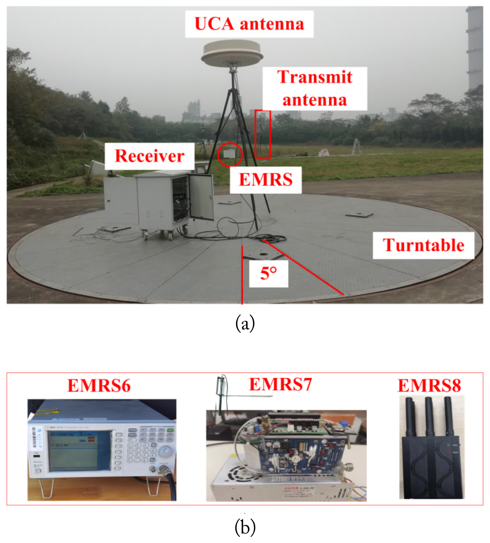
Three actual EMRSs are used to obtain the measured dataset. Fig. 4 shows the experimental scene. A UCA antenna with seven arrays and a receiver is used to collect measurement data from three actual EMRSs. The UCA is above the turntable, with 72 grids and an average interval of 5°. The actual EMRSs and transmit antennas are placed about 20 m away from the UCA, as shown in the red circle and rectangle in Fig. 4(a). The three actual EMRSs are shown in Fig. 4(b), which are the actual signal generator, unauthorized broadcast, and signal jammer, and marked as EMRS6, EMRS7, and EMRS8, respectively. θ6, θ7, and θ8 represent their directions. EMRS6 and EMRS7 are narrowband radiation sources with stable amplitudes. Their frequencies are set to 110 MHz, and the transmit powers are 15 dBm and 150 dBm, respectively. EMRS8 is a broadband radiation source with a stable amplitude that can generate 100–2,600 MHz radiation signals within a radius of 5–20 m. The measured in-phase component/quadrature component (I/Q) sequences are taken as observed signal samples.
The interval of the turntable is 5°, so the direction difference of the three actual EMRSs is set to Δθ1 = {5°, 10°, ···, 50°}. Therefore, 620 I/Q sequence samples are measured when they work together. Moreover, 675 I/Q sequence samples are obtained when any two of them work at the same time.
2. Verification Experiment
The datasets are used to verify the proposed separation method for electromagnetic radiation sources. First, 80% of the samples are used as the training set and 20% as the test set to train and test the PSSNet. The learning rate, epochs, and the number of each batch for the BN layer are set to 0.01, 64, and 1,000, respectively. Fig. 5 shows the training and test loss curves of PSSNet. With the increase in epochs, both the training loss and the test loss gradually converge to a stable value close to 0, which means that the PSSNet is well-trained.
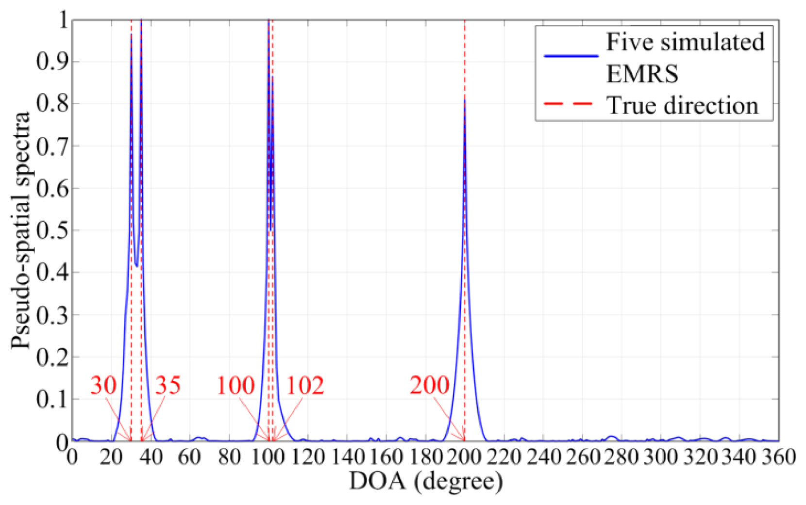
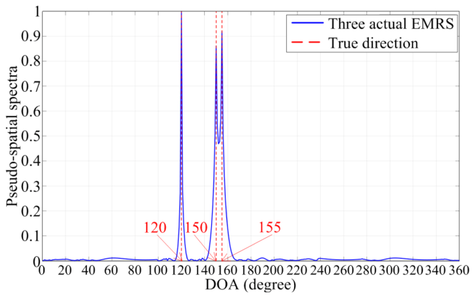
One test sample of the five simulated EMRSs, generated when the directions are 30°, 35°, 100°, 102°, and 200°, the signal-to-noise ratio (SNR) is −5 dB, and the number of arrays (M) is 7, is fed into the trained PSSNet. The results are depicted in Fig. 6. The PSS of the three actual EMRSs with directions of 120°, 150°, and 155° is shown in Fig. 7. As can be observed, PSSNet estimated the PSS well, even when the direction difference between the two sources is 5° or 2°. The spectral peak is a sharp “needle shape,” which is conducive to accurately obtaining the number and DoAs of the radiation sources so as to calculate the mixing matrix.
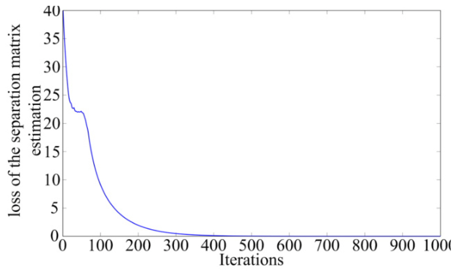
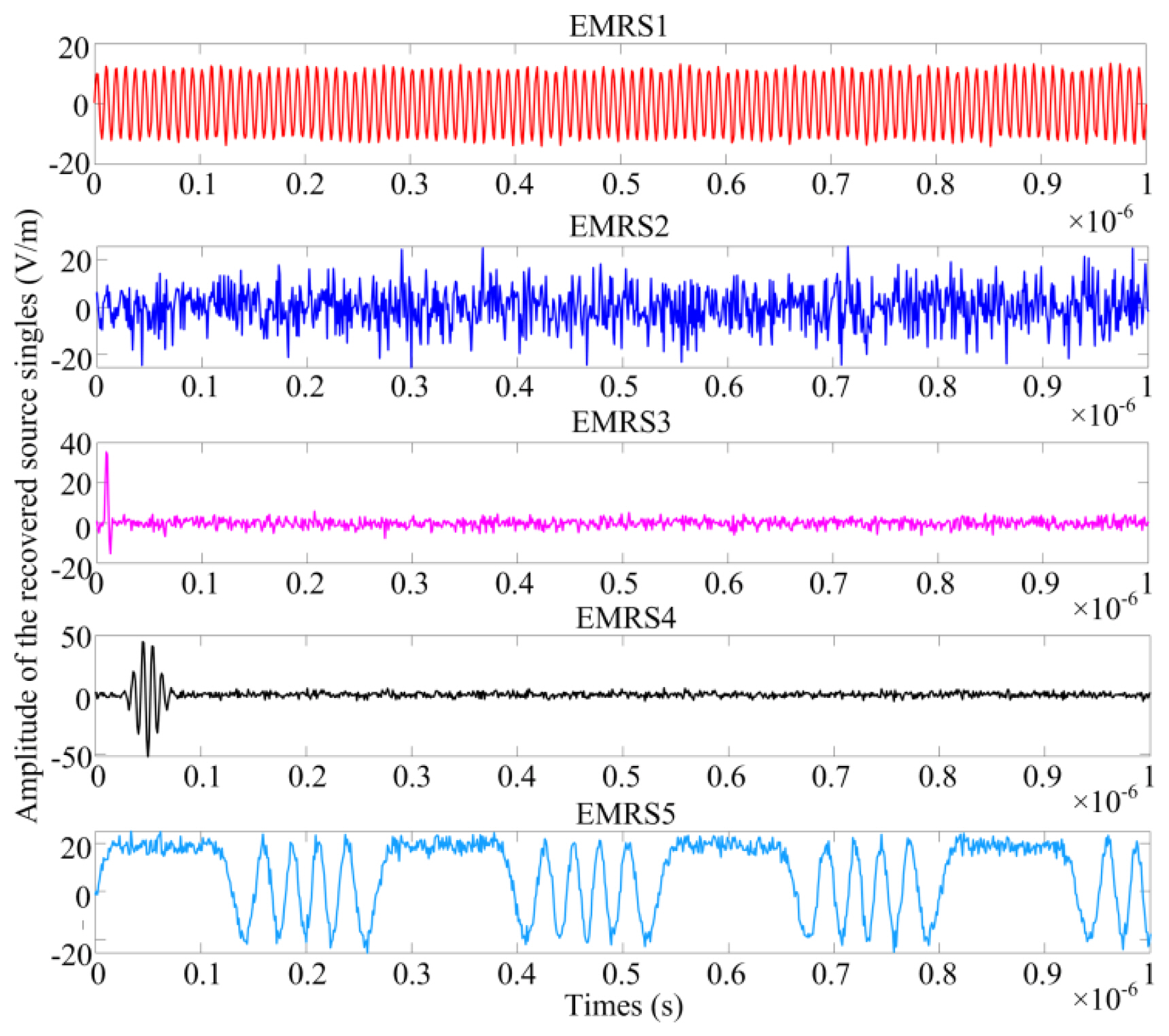
Afterward, the separation matrix is estimated according to the mixing matrix and the loss function proposed in Section IV, and the source signals are recovered. Experiments based on samples from five simulated EMRS are carried out to demonstrate the performance of the proposed loss function and signal recovery. Fig. 8 shows the loss of the separation matrix estimation, which converges stably to 0 after 400 iterations, meaning that the separate matrix is quickly estimated. The five recovered signals are shown in Fig. 9. The time-domain waveform of the recovered signals is similar to that of the source signals shown in Fig. 3.
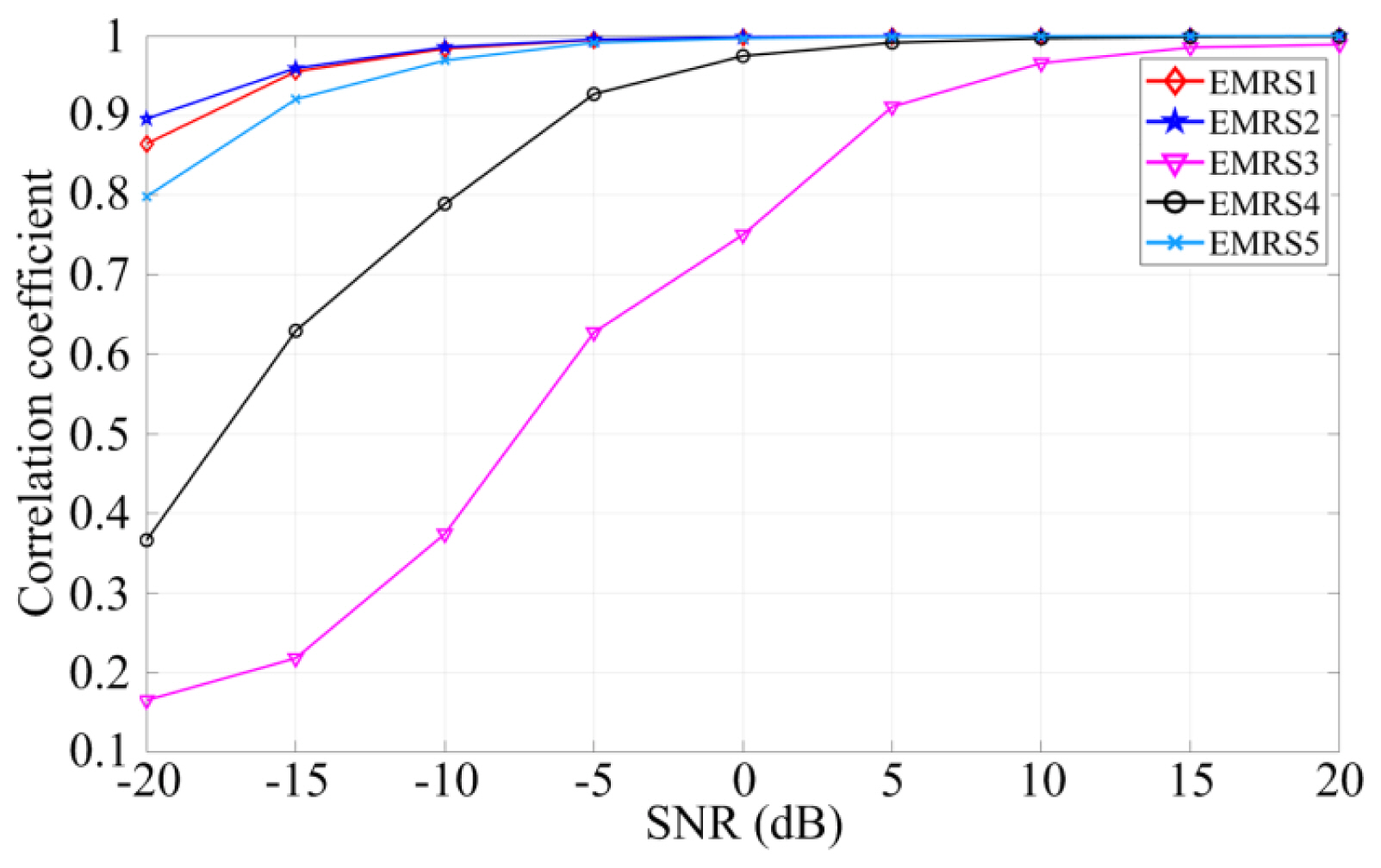
Moreover, the performance of the proposed separation method is inevitably affected by the SNR and M. The CC between the recovered signals and the source signals with different SNRs when M = 7 are shown in Fig. 10, which shows that the bigger the SNR, the bigger the CC. When the SNR is greater than 3 dB, the CC for all EMRSs is greater than 0.8, which means that the proposed separation method can effectively separate the wideband signals as well as the narrowband signals. The separation performance for EMRS3 and EMRS4 is poor, which is caused by the strong correlation between them because they are the same type of EMRS, with a directional difference of only 2°.
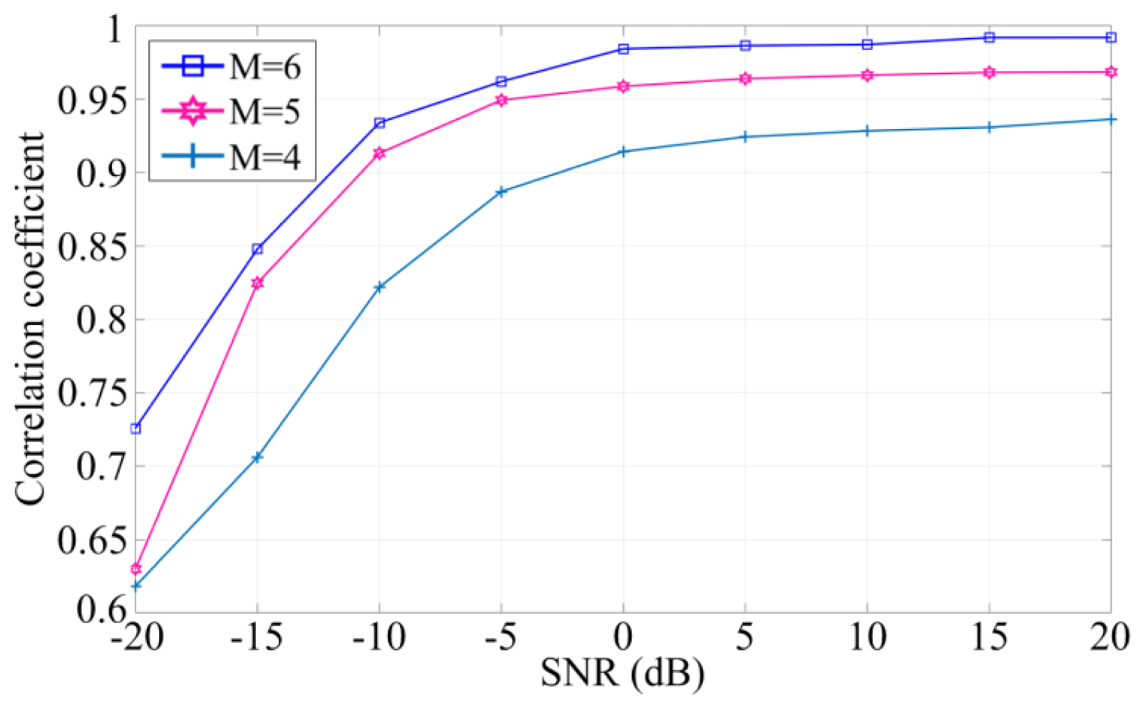
The CC shown in Fig. 11 describes the separation performance of the proposed separation method under different numbers of arrays. This shows that, in the underdetermined case represented by M = 4, when the SNR is greater than −10 dB, the CC is higher than 0.8. Meanwhile, the CC is higher than 0.9 when the SNR is greater than −10 dB in both overdetermined and determined cases. The experiment verified that the proposed method could achieve EMRS separation under various cases.
3. Comparative Experiment
This section illustrates the innovation of the proposed separation method through comparative experiments. On the one hand, the proposed PSSNet was compared with the current popular FC-based network (FCNet) [18] and CNN-based network (ConNet) [19] for DoA estimation. Three networks were trained and tested on the same dataset, whose samples were simulated with an SNR of −5 dB. According to the test results under different numbers of arrays, the RMSE of DoA estimation and number-of-source estimation is shown in Table 1. The training and test times of the three networks under different numbers of arrays are listed in Table 2.
As can be shown, all three neural networks correctly estimated the number of sources, but FCNet and ConNet training preset the number of sources as 7. The RMSE of the DoA estimation of PSSNet is less than 1°, which is smaller than the estimated results of FCNet and ConNet. The time cost of the three networks is independent of the number of arrays. FCNet requires more training and testing time, while ConNet and PSSNet have similar time costs. PSSNet is better at estimating DoA, which reduced the RMSE of the DoA estimation of FCNet and Con-Net by 61.9% and 43.4%, respectively.
On the other hand, the proposed separation method is compared with state-of-the-art FastICA [9] and cluster-based SCA methods [16]. Table 3 shows the CC and RMSE of three methods with different numbers of arrays when SNR = −5 dB. Table 4 shows the running time of three methods with different numbers of arrays when SNR = −5 dB, where the running time of the proposed separation method includes the average training and test time of a sample.
FastICA was used to validate (over)determined cases, and cluster-based SCA was used to validate (under)determined cases. The proposed separation method had the largest CC, the smallest RMSE, and the least running time, which increased the average CC of FastICA and Cluster-based SCA by 9.14% and 12.88%, respectively, and reduced their running times by 27.65% and 40.94%. Its performance is relatively stable and less affected by the number of arrays.
VI. Conclusion
In this study, a separation method consisting of five steps is proposed to separate EMRSs of the same frequency. The proposed PSSNet increased the accuracy of DoA estimation because of the fusion layer. The RMSE of the DoA estimation of PSS-Net was less than 1°. The introduction of a new loss function for separation matrix estimation as the optimization criterion improved performance in recovering source signals. When the SNR exceeded −10 dB, the CC was higher than 0.8 in underdetermined cases and higher than 0.9 in overdetermined and determined cases. The proposed separation method reduced the running time, making it suitable for applications in electromagnetic environment monitoring systems that use array sampling to quickly identify EMRSs of the same frequency.