Time-Domain Measurement Data Accumulation for Slow Moving Point Target Detection in Heavily Cluttered Environments Using CNN
Article information

Abstract
In modern radars, the target detection probability is increased by lowering the detection threshold via signal processing to detect a point target with a small radar cross-section value. However, a lower threshold increases the number of false targets. In the conventional tracking method, which uses a general tracking filter, the measurement data between scans should be compared. Therefore, for a large amount of acquired measurement data, the computational complexity can be reduced by accumulating the acquired measurement data over time, recognizing the target movement as a pattern, and training a convolutional neural network (CNN) model. Here, we propose a method to create a desired target scenario by transfer learning and estimate the target position using the activation map of a binary detector CNN model. The model can detect a target using the actual acquired radar data, and the processing time remains constant, regardless of the number of false alarms.
I. Introduction
Research on radar target detection using artificial intelligence (AI) is being conducted for high-resolution imaging radars, such as synthetic aperture radar (SAR) or high-resolution range profile (HRRP) [1–4]. In this field, existing image detection methods can be easily applied because the processed radar data are provided in image form. Another approach involves target identification and state analysis using micro-Doppler [5–9]. Given that this approach uses high-resolution time-Doppler data, algorithms related to image processing can be applied using a spectrogram with Doppler data as one axis.
Existing hit detection methods widely use the constant false alarm rate (CFAR) to detect hits. CFAR is used in many radars because it can maintain a constant false alarm probability. However, because the CFAR determines the threshold value of a corresponding cell using the values of neighboring reference cells, it is affected when neighboring cells are contaminated by topography or jamming [10].
To solve these problems, several AI methods have been proposed to replace CFAR. Jiang et al. [11] detected a target by learning each feature and creating a 3D cube composed of the range-coherent processing interval (CPI) channel of the received radar signal. Xie et al. [12] extracted target information using a convolutional neural network (CNN) by learning it as an image from an R–D map after a fast Fourier transform (FFT). Wang et al. [13] created and learned R–D maps for various signal-to-noise ratios (SNRs) of input data and detected targets using an M-of-N binary integration. Yavuz [14] revealed cases in which the target exists and one in which it does not exist as an input. Most of these methods use R–D maps to detect hits and cannot detect targets in the time and space domains, which is a disadvantage of the CFAR algorithm. Tilly et al. [15] presented a method for performing detection and tracking by forming tensors of accumulated data over time. However, it is difficult to apply normal radar because it uses a point cloud [16] and requires target features. Therefore, an algorithm for general radars that distinguishes between targets and clutter after CFAR processing is required [17].
Correlation becomes an important issue when tracking targets using hits or plots resulting from CFAR processing. All plots detected by surveillance radar must be associated with plots in other scans through the track-while-scan (TWS) operation. In this process, the amount of computation required for the association becomes very important. In general, multiple scans are performed to determine whether the associated results are accurate or false. Therefore, it is necessary to verify the amount of computation required for multiple scans. Tracking and general association algorithms can be used during this process. When defining a scan as searching for an area once, and assuming that the number of targets per scan is M, comparing the data for N scans requires MN data combinations. Consequently, as the number of targets per scan increased, the total computational cost increased exponentially. To reduce the amount of computation, a correlation boundary was set for each measurement data point, and the calculation was performed by limiting the range associated with the measurement data. If a correlation boundary is used, the number of associations between the measurement data is relatively reduced.
Assuming there are m actual targets among the M measurement data in each scan. If the average number of measurement data points within each correlation boundary is k, then there are M*k associations between the two scans and M*kN−1 associations in N scans. This assumption is simplified, and overlapping associations exist. However, because k < M, the number of associations is reduced compared with the case in which the entire comparison is required (Fig. 1).

N scan measurement data.
A general Kalman filter or αβ filter only needs to compare two states: the previous and the current state. Therefore, m actual data points remained after M*k associations between the first two scans, and M*k associations were required between the second and third scans. If this process is repeated, M*k+(N−1)*m*k associations will be required after N scans. However, if a Kalman-type filter is used, an operation for calculating the covariance matrix and gain per scan is required, along with an algorithm for the initiation and association-determining processes.
Fig. 2 shows the number of computations based on the number of measurement data. As shown in Fig. 2, the existing methods significantly increase the amount of computation as the amount of measurement data increases.
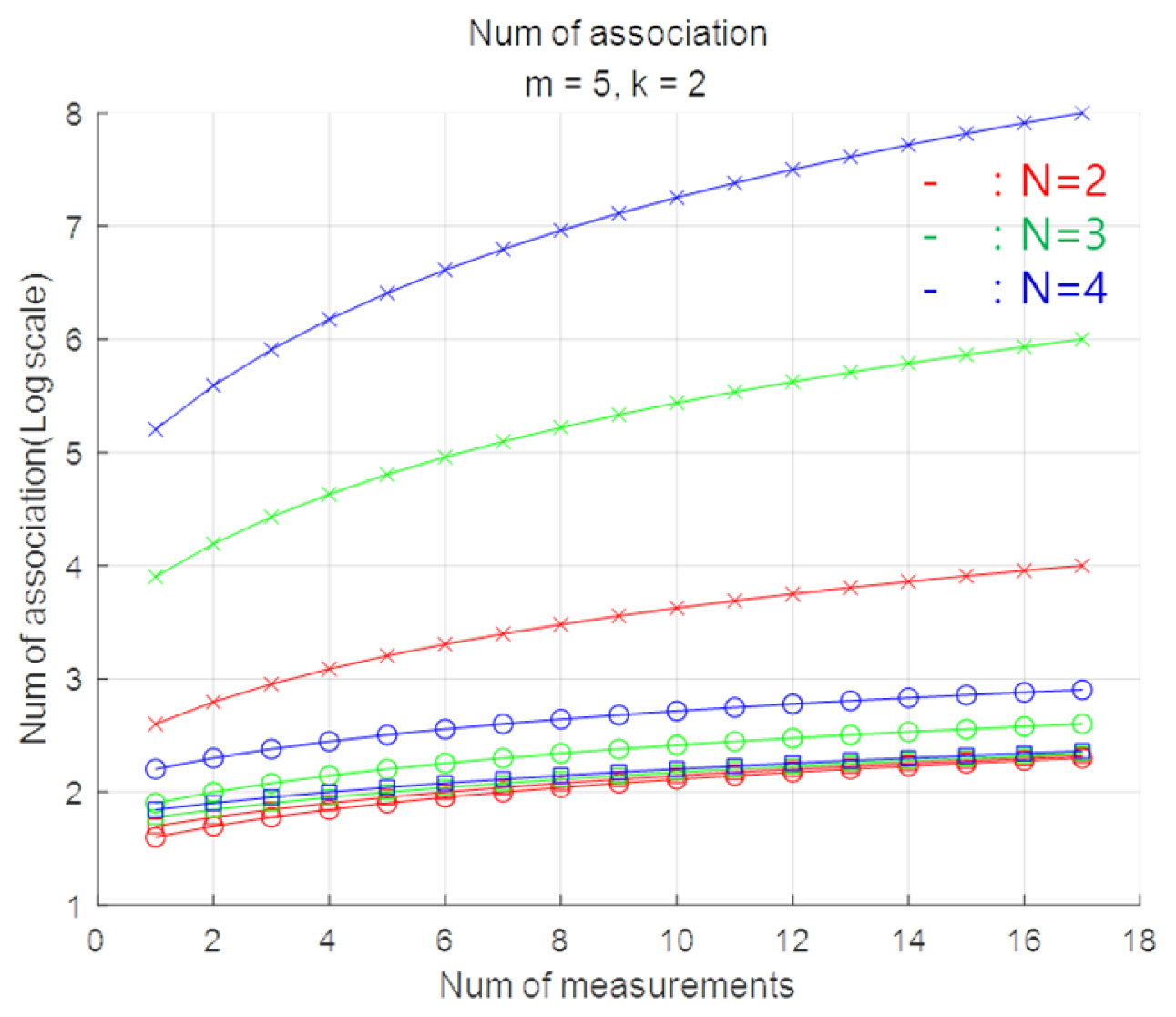
Number of associations (log scale) (x: normal correlation, ○: using the correlation boundary, □: repeating the correlation between two scans).
Therefore, previous association methods are highly sensitive to the amount of measurement data, including clutter and false alarms. Normal radar systems discard data that exceed their processing capacity to prevent system failure, and many conventional processing methods may lose the target information as M increases. Therefore, it is necessary to filter the target information first, such that false alarms are not related to the actual target tracking and the maximum value of the computational amount is fixed.
In this study, we (1) present a method for training a CNN-based model by accumulating data from multiple scans using self-generated low-speed two-dimensional (2D) radar point target data (time-domain measurement data accumulation [TDMA]) to detect a target trajectory from clutter measurement data; (2) form a desired tracking scenario by transfer learning in various cases; (3) estimate the target position by using the activation function; and (4) show that the trained model works well by using real radar data, while the computation time remains constant regardless of the number of the false alarms
II. Simulated Radar Data for Heavy Clutter Situation
When distinguishing a normal target from clutter, velocity, and radar cross-section (RCS) become important features. However, for low-speed, low-RCS targets, these features are no longer the criteria for discrimination.
If the target is sufficiently fast, we can find a moving target by removing the zero-doppler. For large RCS targets, the magnitude-based PDF is sufficiently separated from the PDF of the non-target; therefore, it is easy to increase the detection probability using a threshold and control the false alarm probability to the desired level. However, in the case of a small RCS target, because the PDF of the target and non-target overlap significantly, the threshold to obtain the desired detection probability increases the false alarm probability and generates a large amount of clutter. This clutter becomes individual hit data, resulting in an exponential increase in the progression time of the association process. Therefore, to detect a low-RCS-low-velocity target in the hit domain, a lower threshold in CFAR processing and a robust target detection/tracking method that is not affected by the amount of clutter are required. This is prompted by the radar operator’s method of recognizing a target.
In general, a trained radar operator can check the movement of a target on a radar screen with considerable clutter. The radar operator recognizes the movement of the related moving target in the clutter by detecting the movement of the radar screen over several scans. The degree of movement of the target of the corresponding radar and the movement pattern owing to the measurement error can be learned by the operator trained in the pattern by operating the radar for a long time. This process is shown in Fig. 3.
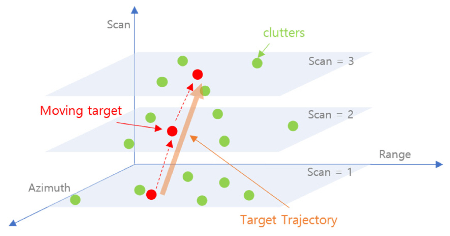
Moving target in the M-scan clutter.
Target detection by a radar operator can be trained similarly to that of the model. For N scans, the clutter information randomly formed on the range-azimuth (R–Az) map, and the target information with a trajectory are formed together. For each scan, the clutter data caused by false alarms that do not originate from the actual targets are independent of the R–Az map. Therefore, the target information is related to each scan, but the clutter data are randomly formed so that they can be distinguished.
When N scans are accumulated, the target information forms a trajectory over time, as shown in Fig. 4(a). This figure shows the movement of the trajectory in each R–D map, where the vertical axis represents the scan. Fig. 4(b) shows a 2D view of this trajectory (data1–data7 refer to each scan, and data8 and data9 refer to the actual target movement). The input accumulated by the scan displays a trajectory representing the movement over time and the location of the randomly displayed clutter. The only difference between the two types of measurement data is whether they form a trajectory or are randomly formed over time; it is assumed that there is no difference in the features of the measurement data.

(a) The 3D and (b) 2D display of moving targets and clutter.
III. Training Data and Model
Several assumptions are required to form a target movement pattern using time accumulation.
1) To learn a pattern, existing image recognition methods can be used only when the target is detected in the 2D domain. Therefore, the radar data are based on the 2D domain (R–Az).
2) The learning effect is reduced for fast-moving targets because the movement of the target must be related to the time required to observe the image. A sufficiently slow target is assumed. In this study, it was assumed that the target did not move more than two cells per scan. However, depending on the capabilities of the radar (such as the size of the range cells) or the speed of the target, there may be more than two cells per scan. In this case, performance degradation may occur.
3) The type of target is not discriminated against, and even a nonmoving detection is considered a target. The detection results, other than the targets, are clutters, which are not correlated with time and are randomly generated from scan to scan.
4) The input for learning excludes terrain; that is, the detection result in the learning area is a target or random clutter.
In this study, N-scan data were generated when generating data for learning. Different scenarios in which the target existed or did not exist were created, similar to [13, 14]. In the existing case scenario, one target and M clutter were generated in each scan, and in the nonexistent case scenario, (M + 1) clutter was generated in each scan. Additional clutters were added to the nonexistent scenario, so that the difference in the amount of measurement data did not differ in the existent/nonexistent scenario. In the existing case scenario, the target trajectories of the range and azimuth were generated as in Eq. (1):
PR and PAz are the generated positions of the target (range/Azimuth). MR and MAz are the ideal target positions for the range and azimuth, respectively. σR and σAz are the error standard deviations for each axis. randn( ) denotes a normally distributed random number.
The vertical*horizontal axes per scan were expressed based on R*Az. As this is based on radar signals, the received data can be used without conversion in the R*Az domain, and the radar has the same measurement accuracy as the acquired data on the range and angle axes. Therefore, the generated input data becomes 3D matrix data in the form of (Range*Azimuth*Scan). In this study, the size of the range/azimuth cell was based on the value of the actual radar system, and the target measurement error used values based on the actual beam width and size. The size of the input data matrix map was set such that the target did not exceed the map during the entire scanning time. In real radar systems, range accuracy is much more accurate than angular accuracy; therefore, it can cover fewer cells in the range direction but requires more cells in the azimuth direction. Therefore, the input data map per scan becomes rectangular, reflecting the normalized accuracy values, as shown in Fig. 5.

Radar accuracy and TDMA model.
The generated 3D matrix data can be expressed as zero for cells without measurement data and as one (or any nonzero integer) for cells with measurement data. The location information of the target should become integer with the value of the Range*Azimuth cell; since it is a point target, one measurement data must be one cell. The value of the cell corresponding to the target position was set to a nonzero value (Fig. 6).

TDMA model input data.
The CNN algorithm shown in Fig. 7 was used as the training network. The pooling layer was excluded from the general CNN. The pooling layer was helpful in terms of the amount of computation because it merged adjacent pixels; however, this model removed the pooling layer because it had to find the location of one pixel.

TDMA input and network model.
The basic options for learning were as follows: stochastic gradient descent with momentum (SGDM) was used as the solver, and the initial learning rate was set to 0.01. The maximum epochs and mini-batch sizes were 30 and 128, respectively. We set the L2 regularization to 0.0001 and the gradient threshold method to L2-norm.
IV. Comparison with the Conventional Time-Domain Accumulated Detection Method
The performances of the trained TDMA model and the existing time-domain accumulated detection method were compared. As shown in Fig. 8, the typical time-domain accumulated detection algorithm compares the number of scans of data related to the correlation boundary among N scans in the same dataset.
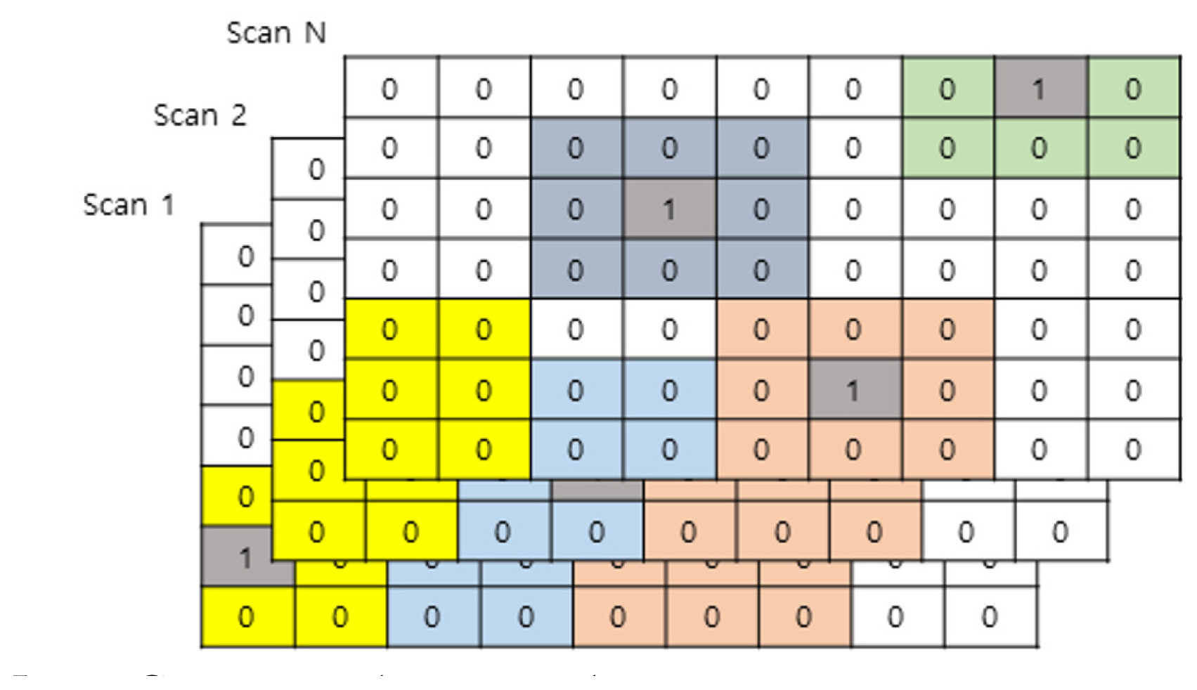
Conventional target tracking.
During N scans, (N, N-1, ..., 1) bundles were selected within the boundary of each measurement data point, and the number of bundles was recorded as a parameter for each bundle.

In the pseudocode 1 results listed, the location of each measurement value and the number of scans of the associated measurement values were recorded. As shown in the pseudo-code, the amount of computation required for the existing time domain detection algorithm operation varies depending on the number of N scans of the dataset and the measurement data.
V. Comparison Results
The performance of the trained model was tested using newly created validation data. The number of scans was set from 3 to 8, and the number of clutters in each scan model was set to [0, 3, 5, 10, 20].
The receiver operating characteristic (ROC) curve in Fig. 9 was drawn by comparing the results determined for each instance in the existing/nonexistent cases. In the case of clutter 0 in Fig. 9(a), almost all discrimination results are consistent with the expected existing/nonexistent case on the input map. The area under the curve (AUC) of Fig. 9 in each TDMA model is as shown in Table 1.

(a) ROC curves according to (a) the number of clutters per accumulated scan and (b) the accumulated scan per clutter.
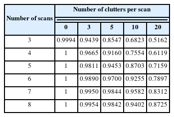
AUC values in each TDMA model
As shown in Table 1, the greater the accumulation of scans, the higher the discrimination accuracy. However, as the number of clutters per scan increased, the accuracy decreased, and the case of 3 scans–20 clutters was hardly discriminated against. Further, as more scans accumulated, the accuracy increased, but the performance improvement rate decreased because of the correlation between the accumulated time and the target movement during that time.
The verification data used in this study were generated using the same method used for the training data. The results of tracking these data using a typical are described below. Each scenario used 6,000 data.
In Fig. 10, each point of the ROC curve of the conventional tracking method is defined as “the number of detections in the correlation area compared to the number of input scans.” When comparing the typical method and the TDMA model using the same data, it was confirmed that the TDMA model showed better performance. In particular, it was found that the detection performance of the TDMA model was maintained to some extent, even when there were many clutters when the TDMA model accumulated sufficient scans, whereas the typical method reduced the performance very quickly when there were many clutters.

Comparison between the TDMA model and conventional model (i.e., conventional tracking method suggested in Section IV): (a) 3 scans accumulated, (b) 5 scans accumulated, (c) 8 scans accumulated.
The computation time in each scan and clutter environment was measured, as shown in Fig. 11. A typical method requires more time as the number of scans and clutter increases. The normalized time ([Computation time] / [Computation time of clutter 0 for each scan]) of each scan increases by a factor of 15. However, the time required by the TDMA model increased only as the number of scans increased, and the time required by the number of clutters did not change. Regarding normalized time, the required time was always the same, regardless of clutter.
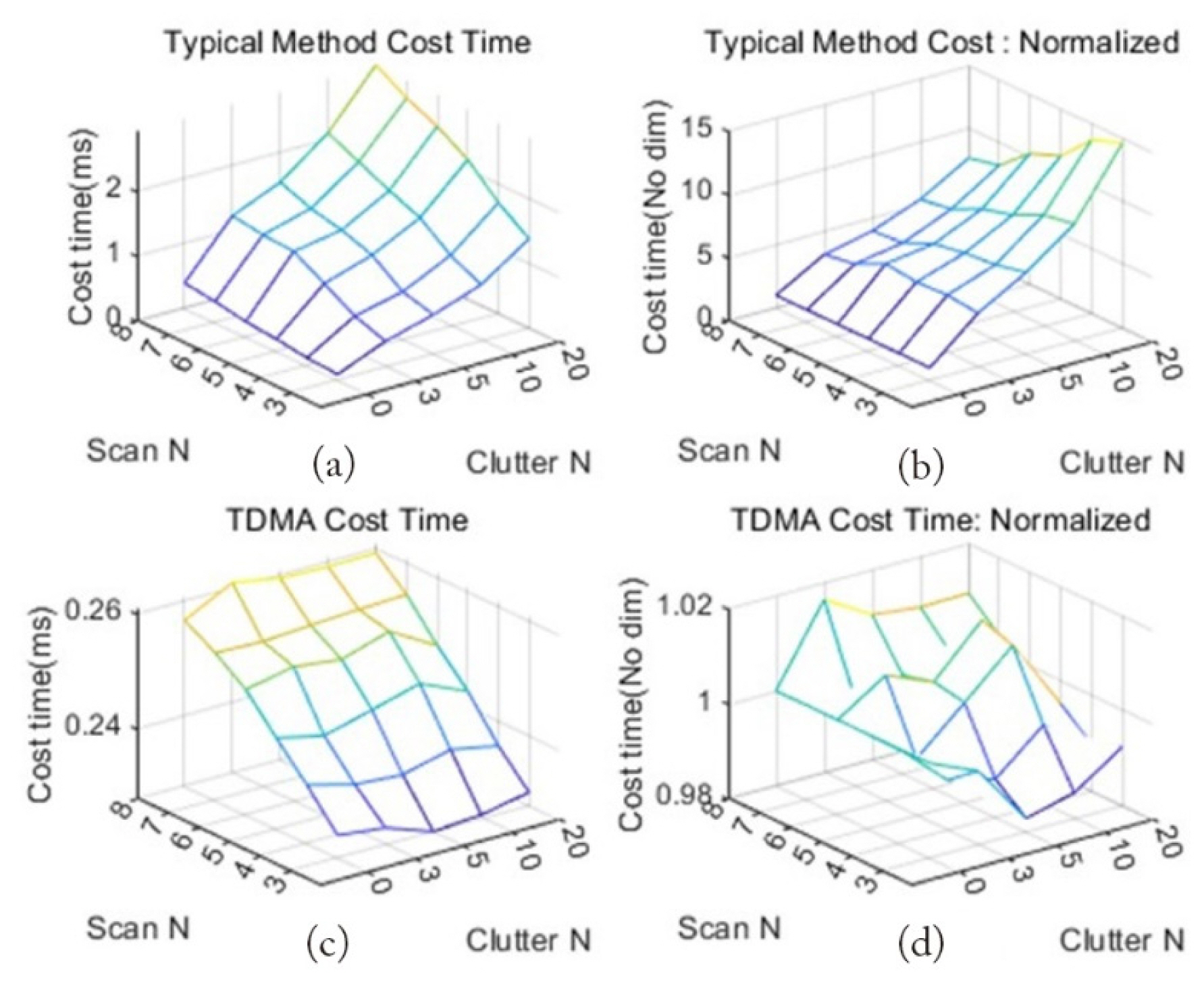
Comparison of the computation time between the two models: (a) computation time of the conventional method, (b) normalized computation time of the conventional method, (c) computation time of TDMA, and (d) normalized computation time of TDMA.
The rationale behind this result is clear. With the TDMA model, the computation time was constant, regardless of the number of clutter or false targets. Therefore, when constructing a system using the TDMA model, the number of false targets or clutter can be significantly increased by significantly lowering the CFAR threshold. This feature is a significant advantage for configuring a system that detects low-RCS targets. Because the processing time is only affected by the number of real targets and the cumulative number of scans, and because these values are design parameters, we can construct a system that can prevent overflow, regardless of clutter or false targets, using a parallel processing design.
VI. Estimation of Target Location using an Activation Map
Given that the TDMA model is a binary detector, only existence/nonexistence was determined. To perform the functions of a typical detector, its location must be estimated. The TDMA model estimates the detection position using the CNN activation map (Fig. 12). The pseudocode 2 was used:

Target detection using an activation map in the TDMA model.

As shown in the pseudocode 2, the last value of the reLU layer (reLU3) in the TDMA model and the weight were multiplied to create an inactivation map, and the position of the peak value was determined using the corresponding activation map. If the amplitude of the peak exceeded the set threshold, it was considered the target. This method enables the discrimination of multiple targets from a single input map.
The activation maps of the existent/nonexistent cases are shown in Fig. 13.
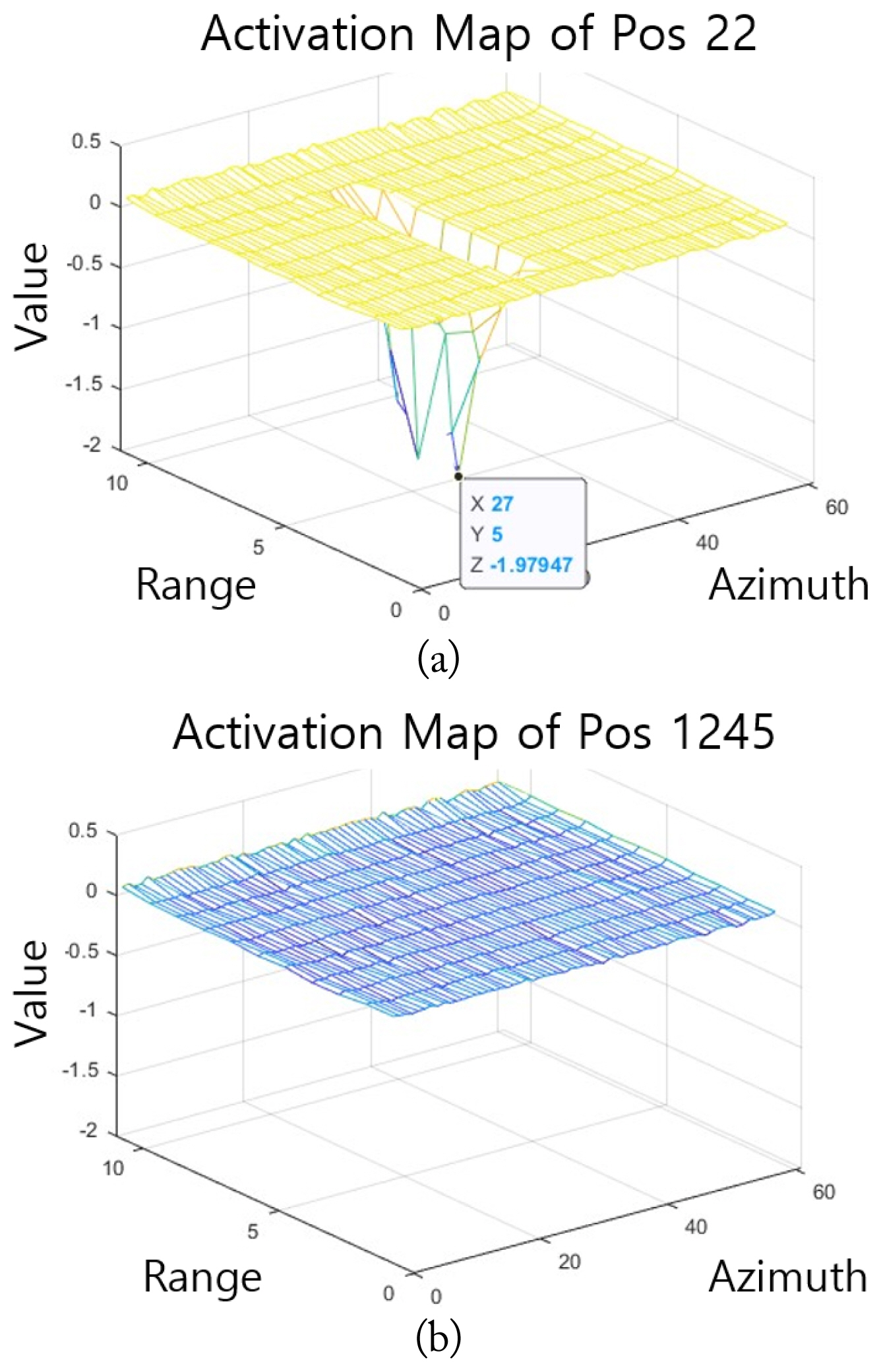
(a) Activation map of the existent case and (b) activation map of the nonexistent case.
To compare the accuracy, the set target position and the determined peak position were compared using verification data. The target position was the validation data, which was the average of the range/azimuth of the cell generated by the target during the N scans. In this comparison, the maximum peak position among the values exceeding the threshold was used to determine one target position per set.
The error value is the cell difference between the estimated peak position and the target position for each axis, as shown in Fig. 14. Therefore, dister, containing both the range and azimuth axes, is defined by Eq. (2).

Cell error and standard deviation for each scan and clutter: (a) position estimation error and (b) error standard deviation.
Cases in which dister was greater than 10 cells were the result of detecting the wrong location in many cases, and the ratio of the entire test (target false detect ratio) was as Table 2.
Target false detect ratios
As the clutter increased and the number of scans decreased, the probability of predicting an incorrect position increased; this was because, as the clutter density increased, the probability that random clutter forms trajectories at different locations also increased (Fig. 15). However, in most cases, the correct position was predicted, and in this case, the error of each axis was less than two cells.

False detect ratio.
VII. Results with Real Data
A TDMA model was used to filter and track the actual radar measurement data. The following training scenario was added to the TDMA model using transfer learning.
1. Input Data Map for Training
The training map size was set as follows: The default training map size was 11 × 61 × 7 pixels. The range and azimuthal cell size were 10 m (total 110 m) and 0.1° (total 6.1°), respectively.
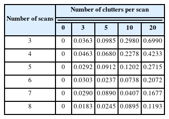
The basic training scenario was as follows: the generated target velocity was 0–15 m/s, and measurement errors of the range axis of 1 m (variance) and azimuth of 0.1° were added. In a low-level clutter scenario, we added clutter at the rates listed in Table 3.

Ratio of clutter N
There were seven accumulated scans, and 8,000 existent/ nonexistent scenarios were used. During the basic scenario training described above, low-clutter and memory-track training were added using transfer learning. For low-clutter training, 1,000 cases in which the clutter and targets were three or fewer in seven scans were trained as nonexistent cases. For memory tracking training, 2,000 cases in which there were five non-detect scan data points among all seven scans were trained as nonexistent cases.
We applied the TDMA model trained as described above to the actual radar measurement data.
2. Measurement Data from Actual Radar
The measurement data from the radar were 2D sea surface data obtained from the East Coast of South Korea. After signal processing, it becomes a point target, and each measurement data point contains only location information, excluding frequency characteristics (Table 4).

Characteristics of real radar data
The obtained radar data were tens of minutes of data, and the marine clutter and target data (stop target, moving target) were mixed (Fig. 16).

Full data of the surface radar data, 2,846 scans.
As the acquired radar data included a large number of scans, data were extracted from seven scans for application to the TDMA model. Of the total data, 65–95 scans were used as the starting scans, and an accumulated input set of seven scans was created for each scan. The number of scans ranged from 65 to 101. The data were extracted in the same manner as shown in Fig. 17.

Data crop for the TDMA model input.
The entire radar data area was divided into cells with a range of 10 m and an azimuth of 0.1°, and this entire area was divided into 11 × 61 × 7 input sets centered on the range of 2–20 km and an azimuth axis of 15–60°. Each area had an overlap of 10 m and 1°, and the entire area was divided into 2010 areas (Fig. 18).

Area separation for the model.
Target tracking was performed using the TDMA model for each area. The results of scan 65 are as follows, and Fig. 19 shows an enlarged part (the dots represent the radar measurement data, and the squares represent the positions estimated by the TDMA). As shown in the Fig. 19, the TDMA model was able to estimate the location of the target trajectory well, and it was confirmed that the measurement data that were not estimated as targets were only one-time measurement data.
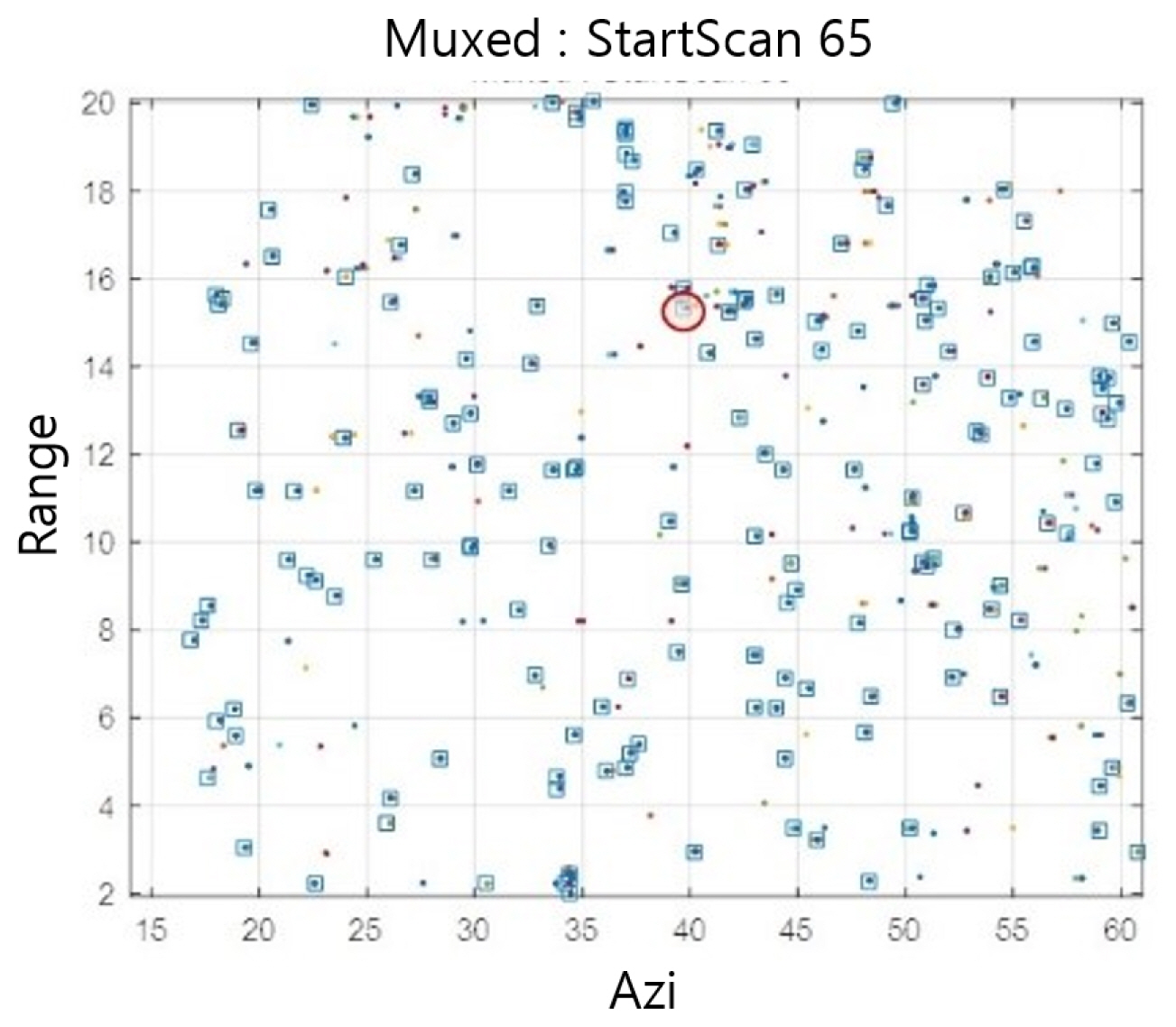
Target detection results using the TDMA model.
The activation map and contour map of the center are shown in Fig. 20. The input data were repeatedly displayed in the same cell because the position of the target was normalized to each cell. Therefore, the measurement data in the contour map in Fig. 20 appear to exist only in the two x-y coordinates during the seven scans. The target positions estimated using this value were similar to the actual positions.

Activation map of the TDMA model: (a) 3D points, (b) activation map, and (c) contour map.
Using the results shown in Fig. 19, we compared the changes in the target detection results according to the activation map threshold. The basic threshold, as shown in Fig. 21, was 0.8. This value was changed to 0.6, 0.4, and 0.2 to compare the number of detected targets and the computation time (Table 5).
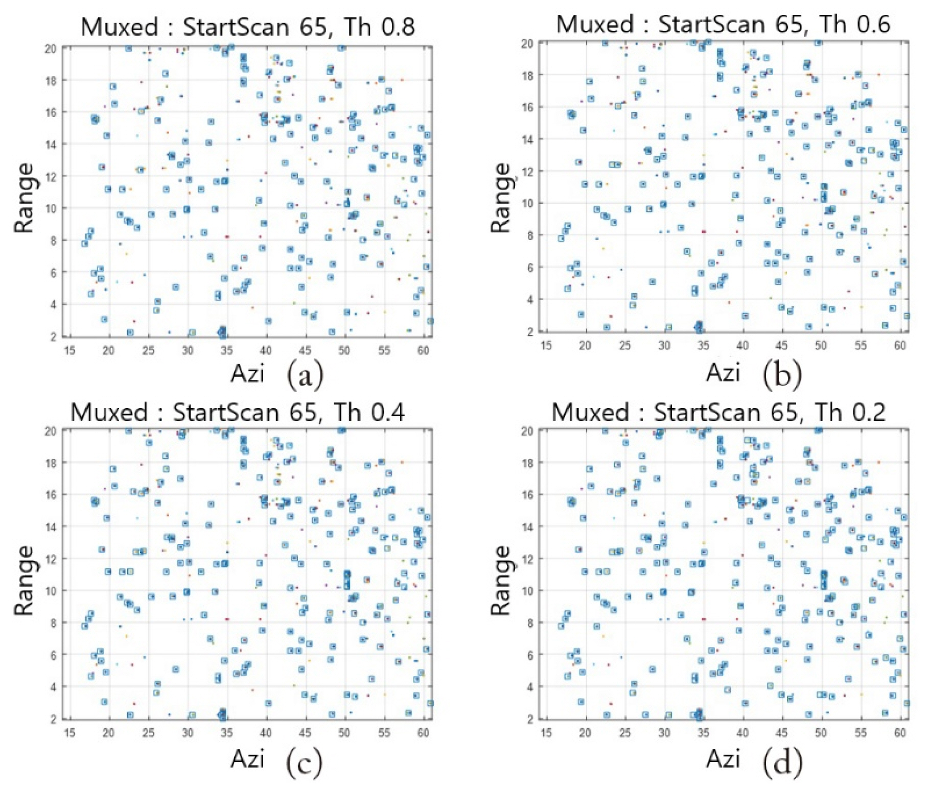
Comparison of detection results according to the thresholds: (a) 0.8, (b) 0.6, (c) 0.4, and (d) 0.2.
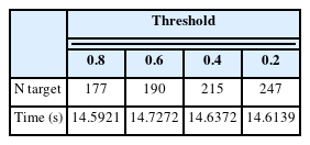
N of detected targets and computation times
As the threshold changed, the target detection sensitivity also changed. However, as the threshold decreased, the number of detected targets increased; however, the computation time did not change significantly.
Next, we analyzed the cases in which the measurement data were increased by adding random clutter to the same radar data, using a method of adding P clutter to the entire area per scan. Therefore, the amount of clutter added over the seven scans was 7 × P.
The changes in the number of targets and the time required were compared according to the results of mixing the clutter. This computation-time comparison was performed using MATLAB on a PC, and there was a deviation every time the program was executed. In real radar systems running with a real-time OS, faster and more even computation times will be needed.
As shown in Fig. 22, even if the added clutter was increased for the same radar data, the total number of TDMA results and computation time did not increase significantly. When more than 2,000 clutters were added per scan, the number of TDMA results tended to increase; however, this is because a large amount of randomly added clutter correlates with each other to form what looks like a trajectory.
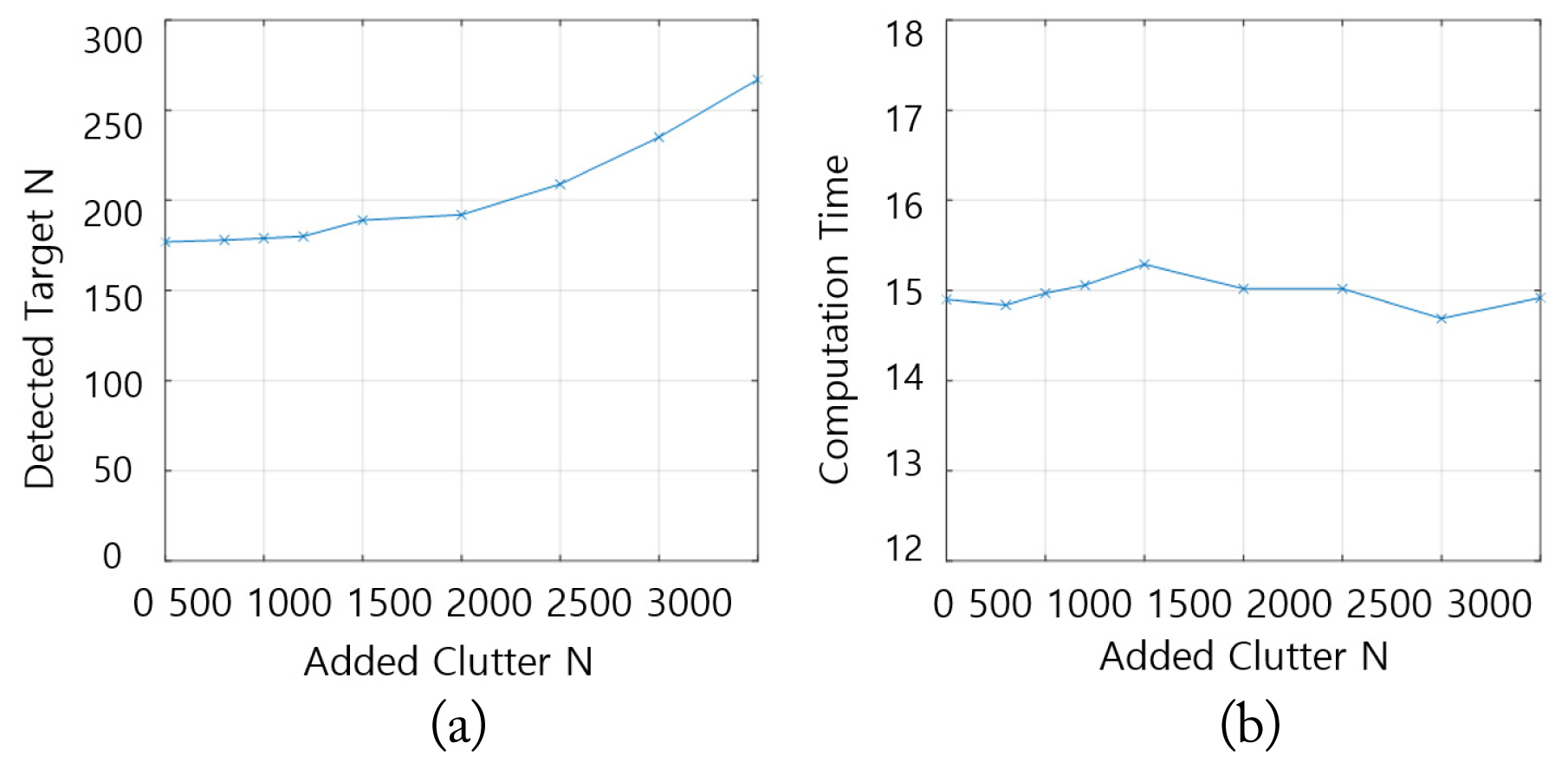
(a) Detected target N and (b) computation time.
The results of tracking the actual radar data at two scan intervals, from scans 65 to 95, are shown in Fig. 23. The actual radar data used were 65 to 101 scans, and the basic radar data and data with 1,000 clutter points added for each scan were detected together using the TDMA model. A total of 37,000 clutter points were added during the 37 scans; however, when compared with the basic radar data, there was no significant difference in the data detected as actual targets.
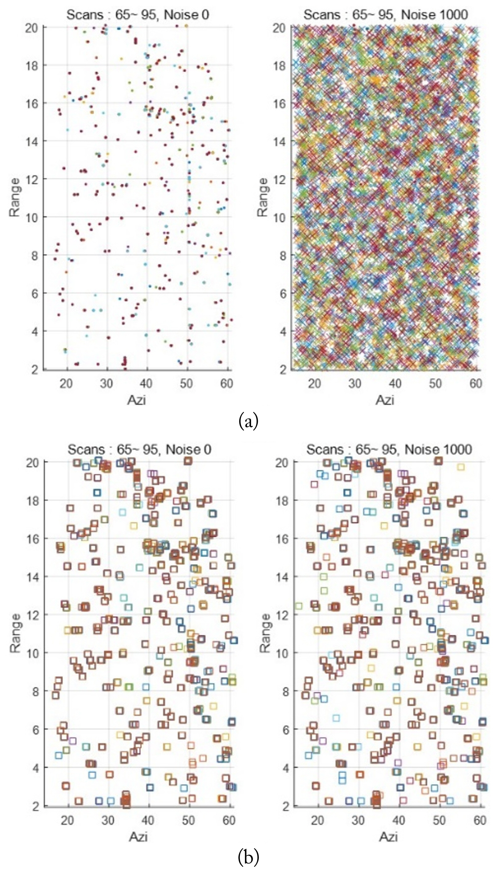
Full-scale target detection for the radar data and clutter-added data: (a) origin data and noise-added data and (b) TDMA results in each case.
VIII. Conclusion
The TDMA model can detect the presence of a target with a higher probability than typical methods, even in the presence of a large amount of clutter. Using the activation map generated in this process, the position of the target can be detected simultaneously; thus, the filtered target data can be provided to a tracking filter. The TDMA model estimated the position of the target with high accuracy, from no clutter to a large amount of clutter, and, above all, showed almost the same accuracy and computation time, even when there were many acquired measurement values. In typical correlation methods, as the amount of measurement data increases, the amount of computation increases exponentially, which can cause system overflow. However, if the TDMA model is used, it is possible to design a system that always operates within the desired time, regardless of the amount of clutter, using parallel processing, which can be very helpful in actual system implementation.
Acknowledgments
This work was supported by the Agency for Defense Development (No. 912975101).
References
Biography

Wonmin Cho
https://orcid.org/0009-0006-9022-5503 received his B.S. degree in Electrical Engineering from Seoul National University, Seoul, Republic of Korea, in 2005 and his M.S. degree in Electrical and Computer Engineering from Seoul National University, Seoul, Republic of Korea, in 2007. Since 2007, he has worked at the Agency for Defense Development, Daejeon, Republic of Korea, where he is currently a Senior Researcher. He is currently pursuing his Ph.D. degree in the Graduate School of Convergence Science and Technology from Seoul National University, Seoul, Republic of Korea. His current research interests include radar control, signal processing, and artificial intelligence.

Nojun Kwak, https://orcid.org/0000-0002-1792-0327 received his B.S., M.S., and Ph.D. degrees in electrical engineering and computer science from Seoul National University, Seoul, South Korea, in 1997, 1999, and 2003, respectively. From 2003 to 2006, he worked with Samsung Electronics, Seoul, South Korea. In 2006, he joined Seoul National University as a BK21 Assistant Professor. From 2007 to 2013, he was a faculty member in the Department of Electrical and Computer Engineering, Ajou University, Suwon, South Korea. Since 2013, he has been with the Graduate School of Convergence Science and Technology, Seoul National University, where he is currently a professor. His current research interests include feature learning by deep neural networks and their applications in various areas of pattern recognition, computer vision, and image processing.