Unified GSTC-FDTD Algorithm for the Efficient Electromagnetic Analysis of 2D Dispersive Materials

Article information

Abstract

I. Introduction

The finite-difference time-domain (FDTD) method has been popularly employed to analyze the electromagnetic (EM) problems in complex media [1–9]. The superiority of the FDTD method includes simplicity, robustness, and wideband analysis via a single simulation. It is very important to choose an appropriate dispersion model for an accurate EM analysis of media, considering dispersion characteristics. Various dispersion models, such as Drude, Debye, Lorentz, quadratic complex rational function (QCRF), complex conjugate pole residue (CCPR), and modified Lorentz (mLor), have been previously proposed to analyze EM propagation in dispersive media. Among the various dispersion models above, the mLor dispersion model is promising because it can unify the various dispersion models and also the computational efficiency of mLor FDTD simulation is superior to other dispersion-based FDTD simulations [10].

However, when using the conventional FDTD method for accurate EM wave analysis of very thin two-dimensional (2D) materials, enormous computing resources are required because a very small FDTD spatial grid should be used. Recently, the generalized sheet transition condition (GSTC) was successfully employed in FDTD modeling for a single-term Drude dispersion model, and it was reported that GSTC-FDTD can efficiently analyze the EM properties of 2D materials [11]. In this work, we present an efficient FDTD formulation for 2D materials with arbitrary dispersion models. Toward this purpose, we propose a GSTC-FDTD formulation based on a multiterm mLor dispersion model. Numerical examples are employed to show the excellence of the proposed FDTD formulation compared to the conventional FDTD method.

II. Modified Lorentz GSTC-FDTD Formulation

Consider that a 2D dispersive material is located at z = Ω in the xy plane of a rectangular coordinate system. A virtual electric FDTD grid, E_x(Ω⁻), or a virtual magnetic FDTD grid, H_y(Ω⁻), is introduced on both sides of z = Ω via the GSTC-FDTD method. The one-dimensional (1D) GSTC-FDTD update equations for E_x and H_y, respectively along the x- and y-directions in consideration of the virtual electric field grid and magnetic field grid, are as follows:

where ɛ₀ and μ₀ indicate the permittivity and the permeability of the free space, respectively. Note that Δt indicates the FDTD time step size, Δz indicates the FDTD grid size along the z direction, k indicates the space index along the z direction, and the superscript indicates the time index. The virtual electric field, E_x(Ω⁻), and the virtual magnetic field, H_y(Ω⁺), can be represented by the GSTC algorithm in the frequency domain (an e^jωt time-dependence assumption) [12, 13] as

where

Note that χ represents the frequency-dependent surface susceptibility tensor, ω is the angular frequency, k₀ is the propagation constant of free space, Δϕξ=ϕξtr-(ϕξinc+ϕξref), ϕξ,av=(ϕξinc+ϕξref+ϕξtr)/2 with ϕ representing the spectral electric or magnetic fields, and the superscripts “inc,” “ref, “ and “tra” denote the incident, reflected, and transmitted waves, respectively [13]. In the FDTD framework, it is necessary to convert frequency-domain relationships (3) and (4) into time-domain counterparts. By applying the inverse Fourier transform (IFT) to (3) and (4) and then applying the central averaging scheme to the resulting time-domain equations, we obtain the FDTD update equations as follows:

Substituting (9) and (10) into (1) and (2), respectively, and rearranging them, we get the following GSTC-FDTD update equations for E_x and H_y:

Let us consider the electromagnetic properties of 2D dispersive materials in the GSTC-FDTD formulation. Toward this purpose, we apply the mLor dispersion model to the GSTC-FDTD formulation. In this paper, for simplicity, we consider only the electrical polarization current density, J˜ee,qxx(ω). Surface susceptibility can be described by the following multiterm mLor parameters:

where a_0,q,a_1,q,b_0,q,b_1,q, and b_2,q are the mLor parameters for the q-th term. Using the multiterm mLor dispersion model for electric surface susceptibility, J˜eexx(ω) in (5) can be expressed as follows:

In the electrical polarization current density for the q-th term, by rearranging (14) and applying IFT, we obtain

By applying FDTD discretization to the above equation, we obtain

By rearranging (16), we obtain the following FDTD update equation for Jee,qxx:

In the above, Ca,q=2b0,qΔt2-8b2,qb0,qΔt2+2b1,qΔt+4b2,q,Cb,q=b0,qΔt2-2b1,qΔt+4b2,qb0,qΔt2+2b1,qΔt+4b2,q, Cc,p=2a0,qɛ0Δt+4a1,qɛ0b0,qΔt2+2b1,qΔt+4b2,q,Cd,q=8a1,qɛ0b0,qΔt2+2b1,qΔt+4b2,q, Ce,q=2a0,qɛ0Δt-4a1,qɛ0b0,qΔt2+2b1,qΔt+4b2,q, and the average electric field component is defined as Ex,avn+1=[Exn+1(k+1)+Exn+1(k)]/2. By considering all multiterm electrical polarization current densities and substituting (17) into (11), we obtain the proposed multiterm mLor dispersive GSTC-FDTD equation for E_x as follows:

It is noted that the FDTD update equation for H_y is the same as the conventional FDTD equation as follows:

In summary, the procedure for the proposed mLor GSTC-FDTD formulation is as follows:

III. Numerical Examples

As proof of concept, in this work, we consider a popular 2D material, graphene, at 10–30 THz. Four-term pole-residue pairs are extracted using the vector fitting technique [14] for the surface conductivity of graphene, as described by the Kubo formula [15].

In this work, μ_c =150 mev, T = 300 K, and Γ=0.5 ps are used for the graphene parameters [16]. As shown in Fig. 1, the surface susceptibility calculated by the vector fitting method is in good agreement with the Kubo formula. Note that both the intraband and interband terms should be considered for the surface conductivity of graphene in the frequency range of interest; thus, a single-term Drude dispersion model-based GSTC-FDTD formulation [11] cannot be employed.

Fig. 1

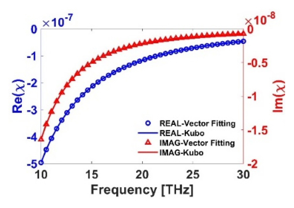
Surface susceptibility of graphene calculated by the Kubo formulas and the vector fitting method.

Table 1 indicates the fitted pole-residue pairs obtained by the CCPR vector fitting method. The first and second pole-residue pairs are real-valued, while the others are complex conjugates. The mLor parameters can be obtained by converting the CCPR parameters by a0,q=-2Re(pqrq*), a_1,q =2Re(r_q), b_0,q = |p_q|², b_1,q =−2Re(p_q), and b_2,q =1 [19].

Table 1

Fitted pole-residue pairs for graphene in the 10–30 THz band

Next, we analyze the EM properties of graphene using FDTD simulations. In FDTD simulations, the 1D computational domain has a physical length of 1,000 nm along the z-direction, and a graphene sheet is located at the center of the computational domain. The entire FDTD domain includes 10-cell perfectly matched layers [17, 18] on both ends. We employ FDTD grid sizes of 1 nm, 2 nm, and 10 nm, and the corresponding FDTD time step size is set for the Courant-Friedrichs-Levy (CFL) stability condition.

A Gaussian-modulated sinewave with a bandwidth of 10–30 THz band is used for source excitation. Fig. 2 shows the reflection coefficient and the transmission coefficient of the graphene sheet. As shown in Fig. 2, the results of the mLor GSTC-FDTD simulation agree well with the theoretical values, regardless of FDTD grid size. However, the mLor FDTD [19] simulations are not in agreement with theoretical results [20] when the FDTD grid is equal to or larger than 2 nm. The reason is why the conventional mLor FDTD simulation for a large FDTD grid size is difficult to model the inside of a graphene sheet with a very thin thickness. However, the proposed mLor GSTC-FDTD simulation can model a very thin graphene sheet with a zero-thickness model; thus, accurate results can be obtained as long as the FDTD grid is about 15 times smaller than the wavelength of the surrounding material.

Fig. 2

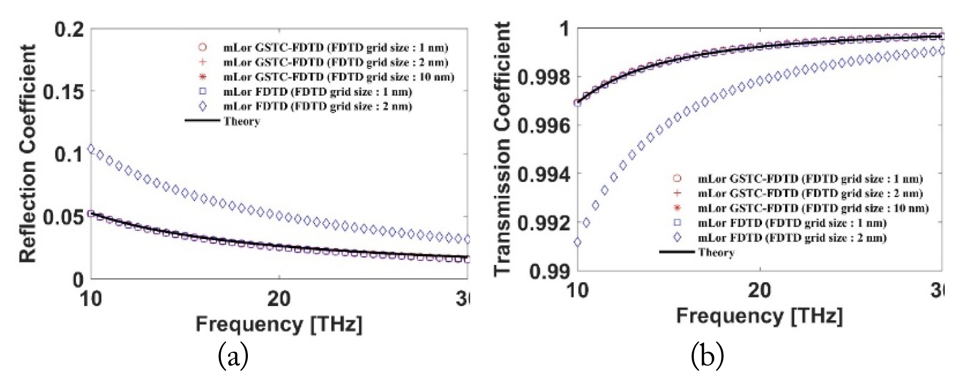
One-dimensional FDTD simulation results of a graphene sheet: (a) reflection coefficient and (b) transmission coefficient.

As the next example, we consider a 2D problem for a graphene sheet, and its geometry is depicted in Fig. 3. We employ the same FDTD grid sizes and the time step size as the 1D problem. The physical size of the computational domain is 1,000 nm × 1,000 nm, and 10-cell perfectly matched layers are considered. The z-directed magnetic current source with a bandwidth of 10–30 THz band is excited at 200 nm above the graphene sheet. The observation point is located at 100 nm below the graphene sheet and H_z is observed.

Fig. 3

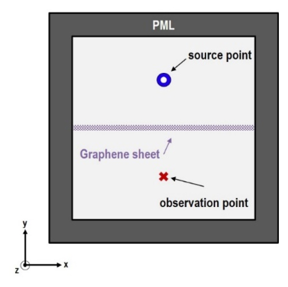
Two-dimensional problem for a graphene sheet.

Fig. 4 shows the normalized magnetic fields of the two numerical results when the FDTD grid size is 1 nm and 2 nm. As shown in Fig. 4, the proposed mLor GSTC-FDTD simulation results are consistent with each other and are the same as the conventional mLor FDTD simulation result for the FDTD grid size of 1 nm. However, the accuracy of the mLor FDTD simulation deteriorates when the FDTD grid size is 2 nm, the same as in the 1D problem. Fig. 5 shows the mLor GSTC-FDTD simulation results when the FDTD grid size is 1 nm, 2 nm, and 10 nm. As shown in Fig. 5, it is observed again that the numerical results of the mLor GSTC-FDTD simulations are the same.

Fig. 4

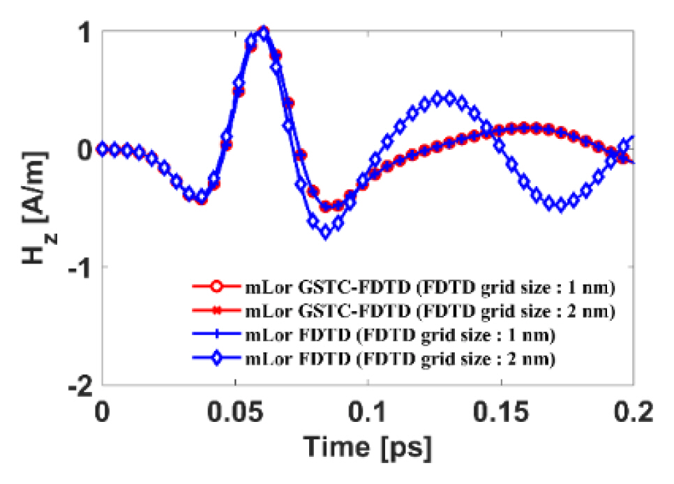
Two-dimensional FDTD simulation results for a graphene sheet.

Fig. 5

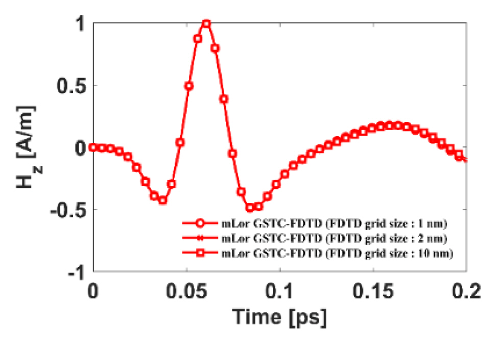
Two-dimensional mLor GSTC-FDTD simulation results for a graphene sheet.

Table 2 summarizes the CPU times and memory storage necessary for accurate FDTD simulations: the mLor FDTD simulation with the FDTD grid size of 1 nm and the mLor GSTC-FDTD with the FDTD grid size of 10 nm. As shown in Table 2, the proposed mLor GSTC-FDTD simulation requires significantly less CPU time and memory storage requirements compared to its conventional FDTD counterpart.

Table 2

Comparison of CPU time and memory storage

IV. Conclusion

In this research work, we propose an efficient and unified GSTC-FDTD algorithm for the EM analysis of 2D dispersive materials. The mLor dispersion model and the GSTC algorithm are employed to derive the proposed FDTD update equations for dispersive 2D materials. It is shown that the surface susceptibility of graphene calculated by the vector fitting method in the THz band agrees with the analytical counterpart. Numerical examples are employed to demonstrate that the proposed mLor GSTC-FDTD formulation can accurately and efficiently analyze the EM characteristic of 2D dispersive media. It is observed that the computational efficiency of the proposed mLor GSTC-FDTD formulation is significantly higher than the conventional mLor FDTD formulation.

Article information Continued

References

Biography
Sangeun Jang received his B.S. degree in electronic convergence engineering from Kwangwoon University, Seoul, South Korea, in 2020. He is currently pursuing the unified course of his M.S. and Ph.D. degrees in electronic engineering at Hanyang University, Seoul, South Korea. His current research interests include computational electromagnetics and nanoelectromagnetics.
Jae-Woo Baek received his B.S. degree from Korea University, Jochiwon-eup, South Korea, in 2015. He received his M.S in 2017 and Ph.D. in 2023 from Hanyang University, Seoul, South Korea. He is currently a postdoctoral researcher at Hanyang University. His research areas are finite-difference time-domain (FDTD), unconditionally stable FDTD, bio electromagnetics, and chiral metamaterials.
Jeahoon Cho received his B.S. degree in communication engineering from Daejin University, Pocheon, South Korea, in 2004 and his M.S. and Ph.D. degrees in Electronic and Computer Engineering from Hanyang Universtiy, Seoul, South Korea, in 2006 and 2015, respectively. From 2015 to August 2016, he was a postdoctoral researcher at Hanyang University. Since September 2016, he has worked at Hanyang University, where he is currently a research professor. His current research interests include computational electromagnetics and EMP/EMI/EMC analysis.
Kyung-Young Jung received his B.S. and M.S. degrees in electrical engineering from Hanyang University, Seoul, South Korea, in 1996 and 1998, respectively, and his Ph.D. degree in electrical and computer engineering from Ohio State University, Columbus, USA, in 2008. From 2008 to 2009, he was a postdoctoral researcher at Ohio State University, and from 2009 to 2010, he was an assistant professor with the Department of Electrical and Computer Engineering, Ajou University, Suwon, South Korea. Since 2011, he has worked at Hanyang University, where he is now a professor in the Department of Electronic Engineering. His current research interests include computational electromagnetics, bioelectromagnetics, and nanoelectromagnetics. Dr. Jung was a recipient of the Graduate Study Abroad Scholarship from the National Research Foundation of Korea, the Presidential Fellowship from Ohio State University, the Best Teacher Award from Hanyang University, and the Outstanding Research Award from the Korean Institute of Electromagnetic Engineering Society.