Implementation Possibilities of Standard Site Method Sub-cases for EMC Antenna Calibrations in Non-ideal Site Conditions
Article information
Abstract
Today, a number of engineering issues require electromagnetic compatibility (EMC) tests, in turn triggering the need for EMC-antenna calibrations. In this framework, experimenters seek accurate and time-saving solutions. Basically, standard site method (SSM) ANSI C63.5-2006 stipulates the near-to-ideal conditions on an empty and vast land, where three antennas are used for antenna factor determination. In our previous work, we investigated the suitability of narrow test sites for antenna calibration according to three-antenna SSM-ANSI-C63.5-2006, whose usability was validated under certain conditions. In the present study, we expand our research by applying the sub-cases of using a known antenna and identical antennas specified in the standard in order to shorten the calibration process. The results reveal that the methods for various calibrations are useful for successfully running the process even in non-ideal sites and help significantly reduce the experimentation time, considering the uncertainty limits specified in EMC test standards.
I. Introduction
Electromagnetic compatibility (EMC) tests are primarily required to ensure the safe use of almost all electrical/electronic devices. The high demand for these tests also significantly triggers the need for EMC antenna calibrations. Among various specifications of EMC antennas, the antenna factor (AF) is the prominent feature of interest. Antenna calibration can basically be defined as AF determination in a specified frequency range. Relevant standards define the methods for identifying AFs and thus performing antenna calibrations. In this context, the standard ANSI C63.5-2006, which this study refers to and whose last update is ANSI C63.5-2017, describes the antenna calibration methods and requirements within the frequency range of 30 MHz–1 GHz [1].
The standard site method (SSM) is based on the study of Smith [2]. In the study, the author proposed to find AFs using site attenuation measurements in an open area test site (OATS).
Measurement accuracy depends on site quality. The SSM stipulates near-to-ideal conditions for the OATS in terms of site dimensions. Furthermore, the basic methodology requires three antennas for antenna calibration. As the first requirement regarding site size limits the prevalence of calibration centers, experimenters seek alternative solutions to circumvent this strictness. In this context, the main approach is to use semi-anechoic chambers (SACs) and fully anechoic rooms (FARs). As an example, Seki et al. [3] devised a method capable of calibrating antennas in SACs with accuracy equivalent to that in the OATS. Our previous study also investigated the suitability of relatively narrow test sites for antenna calibration [4]. We aimed to leverage globally distributed OATSs that are used by companies and labs for the EMC testing of products but are not utilized for EMC antenna calibrations. In [4], we obtained some useful points that will prompt experimenters to consider various aspects when performing calibrations at non-ideal sites. There are even studies in the literature in which researchers have designed specific antennas for EMC tests to overcome the problem [5–7].
The second requirement, the need for three antennas for calibration, significantly extends the time for the entire procedure. To shorten the process, the most featured method is the use of standard/reference antennas. As an example, Meng and Alexander [8] proposed a new way to measure the free-space AF of biconical antennas over 30 MHz to 300 MHz using the standard antenna method (SAM). The study carried out by Sapuan et al. [9] focused on the calibration of the AF of a direct-feed biconical antenna in a SAC using SAM. Another study in this field is that by Amer et al. [10], in which the authors performed antenna calibration in EMC-SAC using SAM and the SSM.
The standard antenna method requires two measurements for antenna calibration. Therefore, although this method significantly reduces the calibration time compared with the SSM, there is a chance to further improve the calibration speed. Some studies show that the AF can be calculated with only one measurement. In [11] and [12], the authors proposed methods to obtain the gains of transmitting antennas, which require only one-time measurement with two antennas. The work in [13] focused on validating the compact-standard antenna method for antenna calibration above 1 GHz, again with just one measurement.
In this context, besides the main three-antenna method, two sub-cases are defined in SSM-ANSI C63.5-2006 to perform antenna calibration with only one site attenuation measurement using two antennas [1]. These are as follows:
The SSM sub-case with a known antenna: This is the case in which there is already an antenna with known AFs. Such an antenna has a valid calibration certificate from a relevant laboratory or manufacturer.
The SSM sub-case with identical antennas: This sub-case refers to the calibration process of an equivalent antenna set, for which the AFs will be determined. Clearly, it is practically impossible for any two antennas to be exactly the same. However, in practical applications, some structures as in the two antennas in a set of precision half-wave dipole are considered nearly identical, having nearly the same AFs.
In this study, SSM sub-case-1 is applied for biconical and log-periodic antennas in the frequency range of 30 MHz–1 GHz, and the results are compared with the classical SSM results. The AF values of the known antenna are obtained from the calibration certificates of the reference institute, TUBITAK-UME (the Turkish Scientific and Technological Research Council-National Institute of Metrology). The calibration uncertainty for sub-case-1 is directly related to the calibration accuracy of the known antenna, as stated in the studies of FitzGerrell [14] and Taggart and Workman [15] about SAM. These two studies are also referenced in ANSI C63.5-2006 and ANSI/IEEE Standard 149-1979 [16].
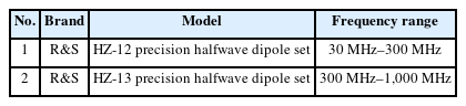
For the application of sub-case-2 in our study, we used a half-wave dipole set, and the calibration results were compared with the data/specs provided by the manufacturer, Rohde & Schwarz (R&S), for the 30 MHz–1 GHz frequency range.
All measurements in this study were performed at the OATS of the Turkish Standards Institution, which was also used for the study in [4]. As highlighted earlier, this OATS is not an ideal site for antenna calibrations given its size, and neither is it a FAR. It is generally used for the EMC testing of products. Thus, this study focuses on the possibilities of EMC antenna calibration using the SSM with a single site attenuation measurement in non-ideal (narrow) sites. The results, together with the uncertainty calculations of the sample calibration processes, are interpreted based on related standard conditions.
To ensure the order of the study in line with the highlighted purpose, we first describe the test method and setup in Section II. In Section III, we provide the experimental results. In Section IV, we draw our conclusions and discuss the practical applicability of the methods used on the basis of the conditions specified in the related standards.
II. Test Method and Setup
The antenna test site (OATS), the control room, and the test setup used for this study are presented in Figs. 1 and 2 [4].
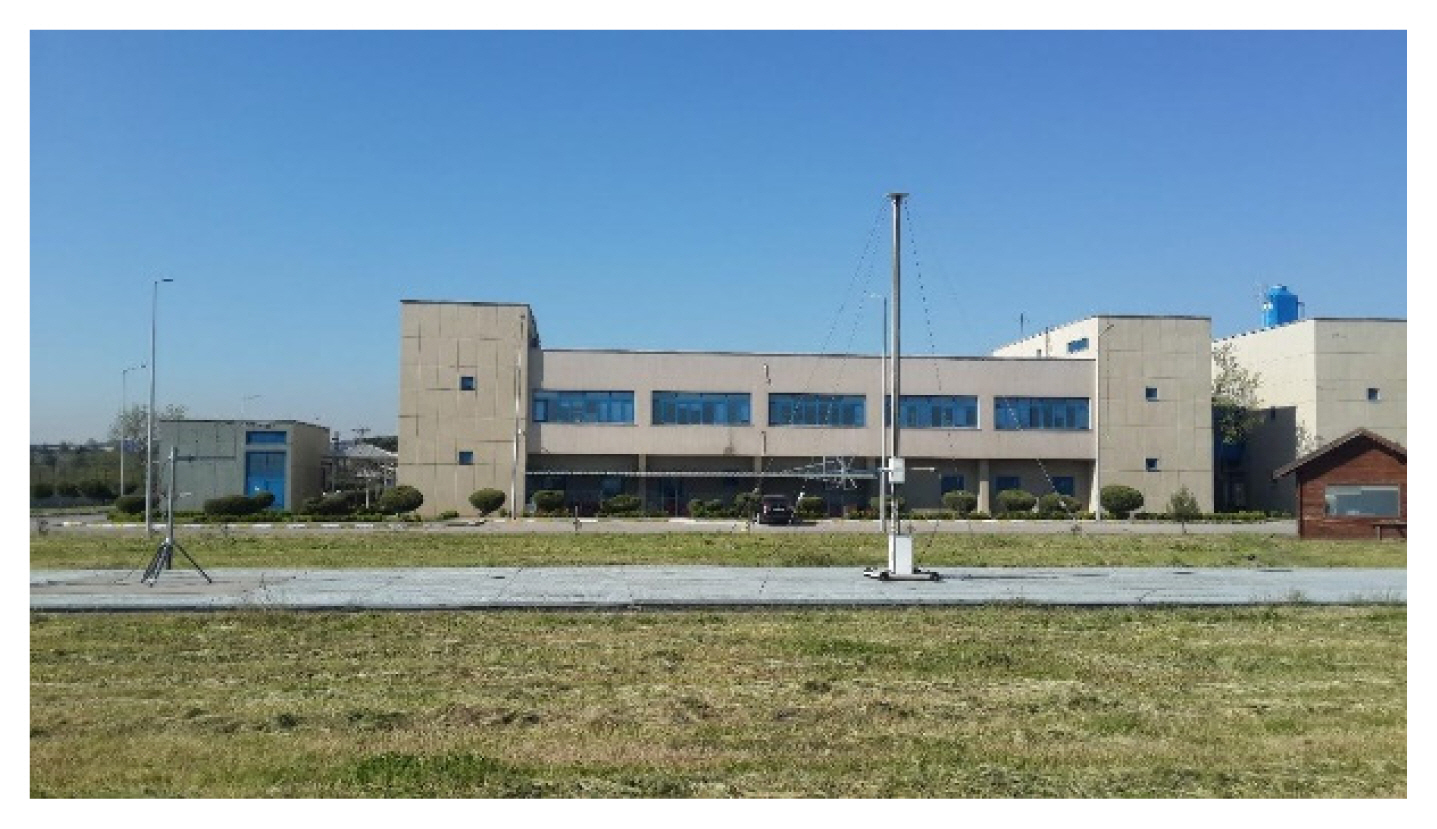
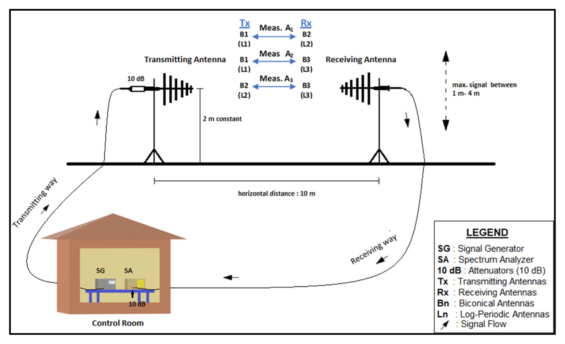
As stated in Section I, the OATS is non-ideal in terms of its dimensions. The basic physical features of the OATS are listed in Table 1. In Fig. 3, the application of all three methods (classic SSM and the two sub-cases) for site attenuation measurements is presented comparatively.

Basic physical features of the OATS

SSM applications: with (a) classic with three antennas (classic), (b) a known antenna, and (c) identical antennas (sub-cases).
In the following sub-sections, we briefly recall the classic three-antenna SSM and provide explanatory information about the sub-cases.
1. The Classic SSM with Three Antennas (SSM-3A)
The antenna calibrations according to the classic SSM of ANSI C63.5-2006 with three antennas are performed, as described in [4] and as briefly mentioned in Section I. The antennas used in the experiments are listed in Table 2. The biconical antenna B3 and the log-periodic antenna L1 are the ones tested. We note that the other study included the calibrations of antennas B2 and L2, which are different from those in this study. All the other instruments and components in both studies are the same. The test geometry is depicted in Fig. 2.

Antennas and instruments used in the calibration processes (SSM-3A and SSM-KA)
With the use of three antennas (Bn: biconical, Ln: log-periodic, n = 1,2,3) and with three site attenuation measurements performed (An, n = 1,2,3), the AFs of the antennas B3 and L1, together with those of the two other biconical and log-periodic antennas (AFn, n = 1,2,3), are obtained using the following three equations in accordance with the classical application of the SSM in ANSI C63.5-2006:
where fM is the frequency in MHz, and
2. The SSM Sub-case with a Known Antenna (SSM-KA)
For the SSM with a known antenna, Eq. (4) can be used to measure the AF according to ANSI C63.5-2006 [1]:
Actually, this equation can be derived by adding Eqs. (1) and (2) side by side. Here, AF1 is the AF of the antenna under calibration (AUC), whereas AF2 stands for the AF of the known antenna. Therefore, only one site attenuation measurement, A1, between two antennas is sufficient to determine the AF of the AUC.
In this study, for the biconical antenna calibration, R&S HK116 biconical antenna (antenna B3 in Table 2) was the one to be calibrated, whereas R&S HK116 biconical antenna (antenna B2 in Table 2) served as the known antenna. The latter has a calibration certificate from the reference institute (TUBITAK-UME). For log-periodic antenna calibration, R&S HL223 logperiodic antenna (antenna L1 in Table 2) was the one to be calibrated, whereas R&S HL223 log-periodic antenna (antenna L2 in Table 2) was the known antenna, which also has a calibration certificate from the reference institute. Some AF values from calibration certificates (AFref) are presented in Table 3 for both log-periodic and biconical antennas (the known antennas). In the certificates, expanded measurement uncertainties were given as 1.50 dB for both antennas.

Certificate antenna factor (AF) values of the known antennas
Except for the antennas, the rest of the instruments used in this calibration process are the same as those in the three-antenna case (Section II-1).
3. The SSM Sub-Case with Identical Antennas (SSM-IA)
In case the two antennas in Section II-2 are identical that they have approximately the same AFs (AF1 = AF2 = AF), Eq. (4) can be arranged as Eq. (5):
Here, A denotes the site attenuation between the transmit and receive antennas.
It is certain that no two antennas can be exactly the same. However, some structures, such as the antennas of dipole sets, show nearly identical characteristics. In such cases, AF in Eq. (5) will be the geometric mean (in linear units) of the AFs of the antenna set members. This situation is also stated in ANSI C63.5-2006, in which Eq. (5) can be used to determine the AF of identical antennas by performing only a single site attenuation (A) measurement between the transmit and receive antennas.
The dipole sets calibrated in this study by applying SSM-IA are listed in Table 4. The set numbered 1 (Model HZ-12) is used in the 30 MHz–300 MHz frequency range, whereas the set numbered 2 (Model HZ-13) is used for the calibration in the frequency range of 300 MHz–1,000 MHz.
Antennas used for calibration (identical antennas)
Before the experiments were started, the site was validated considering possible interference [4].
III. Experimental Results
Below, we present the comparative experimental results of all three methods, namely, the SSM with three antennas (classic) (SSM-3A), a known antenna (SSM-KA), and identical antennas (SSM-IA).
1. Comparative Results of SSM-3A and SSM-KA
The calibrations of the biconical antenna HK 116 (B3 in Table 2) and the log-periodic antenna HL 223 (L1 in Table 2), both from R&S, were performed using both SSM-3A and SSM-KA.
The experimental results are given in Tables 5 and 6 as follows:

Measurement results for the biconical antenna (SSM-3A and SSM-KA)
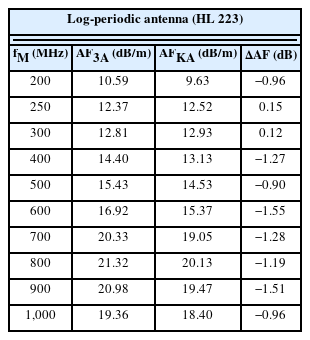
Measurement results for the log-periodic antenna (SSM-3A and SSM-KA)
AF3A for SSM-3A
AFKA for SSM-KA
ΔAF = AFKA–AF3A
The results are also graphically shown in Figs. 4 and 5, respectively.
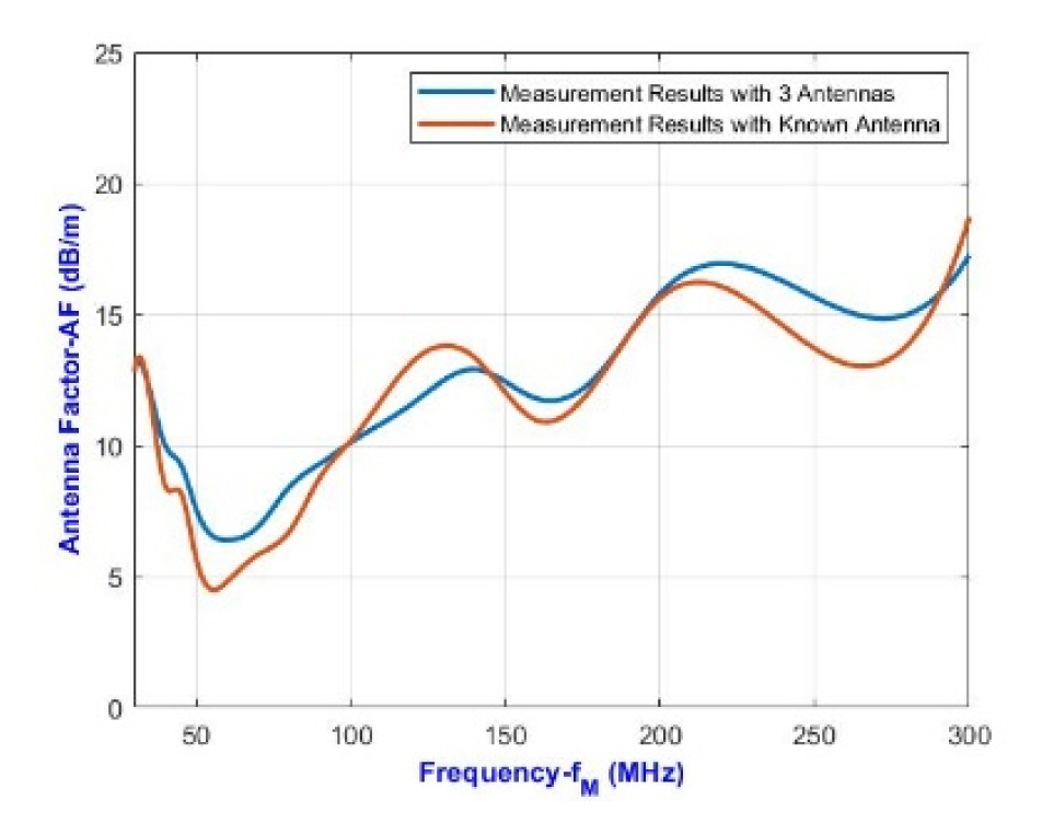
Comparative calibration results of the biconical antenna (SSM-3A and SSM-KA).
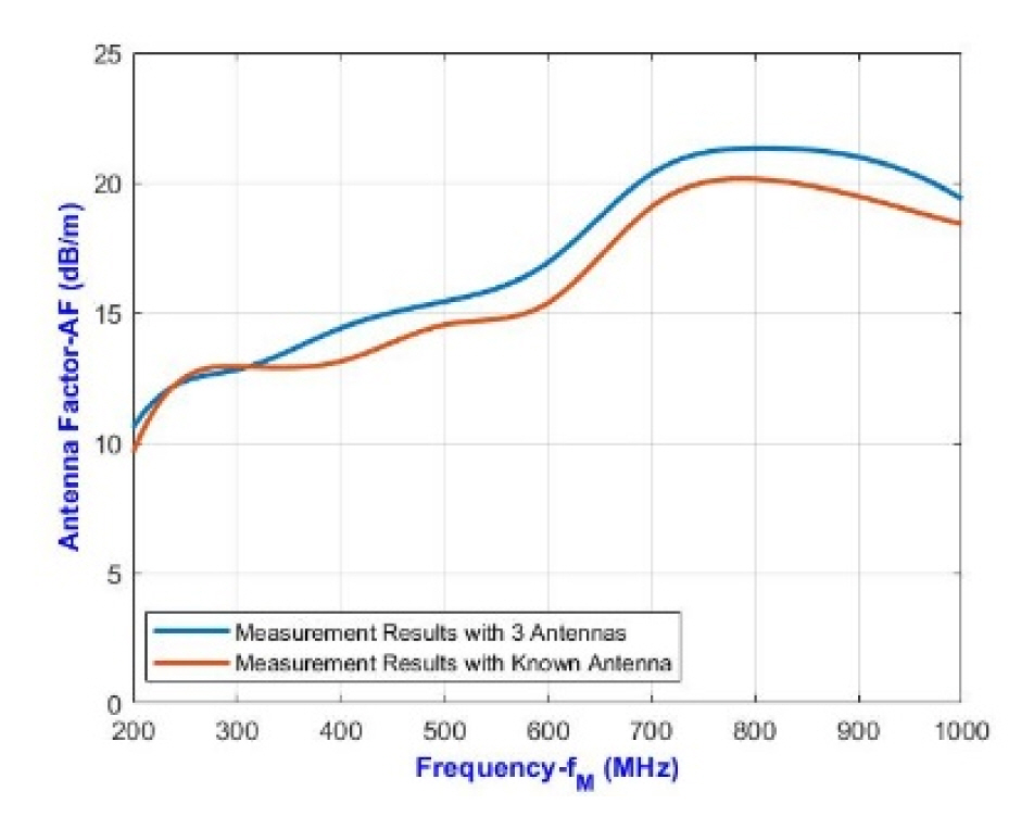
Comparative calibration results of the log-periodic antenna (SSM-3A and SSM-KA).
In Table 5 and Fig. 4, we observe similar behavior in terms of the results for SSM-3A and SSM-KA for biconical AUC across the entire frequency range. However, some differences stand out. The maximum absolute difference between the two cases is calculated as 1.96 dB.
In Table 6 and Fig. 5, the results of SSM-3A and SSM-KA are compared for the log-periodic antenna. We observe a parallel trend of the results with some offset. The maximum absolute difference between two cases reaches 1.55 dB.
The uncertainty calculations in the measurements are conducted according to two basic documents in this field [17, 18].
Assuming that the parameter uncertainties are uncorrelated, the absolute squared combined uncertainty in a result r calculated as r = f(x1, x2, …, xN) is expressed as:
where u(xi) denotes the absolute uncertainty of the parameter xi. The expanded measurement uncertainty U(r) is calculated as in Eq. (7), where k is the coverage factor.
Data on uncertainty budgets are presented in Table 7. For the classical method SSM-3A, a detailed uncertainty analysis was conducted in [4]. In Table 7, we once again present the main components involved in the calculation of the combined measurement uncertainty for SSM-3A. In the table, uAj (j:1–3) represents the combined uncertainty in site attenuation measurement, usite stands for the uncertainty contribution because of site imperfections, and uσ is the repeatability in the overall AF calculation. We note that in [4], to indicate the site quality, we defined the uncertainty component usite, determined as the highest standard deviation of the results from normalized site attenuation measurements across the entire frequency range. It is also worth emphasizing that the related parameter does not appear in the expression that gives the AF, but it is indirectly effective in determining the true value of the AF [4].

Uncertainty budgets for SSM-3A and SSM-KA
For SSM-KA, by applying Eq. (6) to Eq. (4), the combined uncertainty uAF–KA = u(AF1) can be determined as in Eq. (8). Here, we note that in Eq. (4), the parameters fM, A1, and AF2 have individual uncertainties, and, thus, partial derivatives of AF1 exist only with respect to these parameters. In Eq. (8), the value of ufM, which is defined as the uncertainty in frequency, is at a negligible level alongside other uncertainty components and is therefore not included in Table 7. The values for uA1 and usite remain the same as in SSM-3A because the same site is used with the same instrumentation. UREF = k · u(AF2) is the expanded measurement uncertainty of the known antenna, which is given in its calibration certificate. We note that u(A1) in Eq. (8) includes both the measurement uncertainty of site attenuation measurement (uA1) and site contribution in uncertainty calculation (usite), yielding
Regarding the measurement uncertainties of the two methods, SSM-KA is supposed to have the advantage of only one site attenuation measurement. However, because of the dependency on the uncertainty of the known antenna, which is stated as 1.50 dB (for k = 2) in its calibration certificate, the overall expanded measurement uncertainty UAF–KA is found to be 1.89 dB, which is higher than UAF–3A calculated as 1.20 dB. An examination of the comparative measurement uncertainty calculations in Table 7 clearly reveals that the uncertainty of the known antenna heavily predominates among all contributors. This indicates that with known antennas that have lower measurement uncertainty, the overall measurement uncertainty of the method can be significantly reduced.
As a result, SSM-KA can be used for antenna calibration depending on the application in which the respective antenna will be used, the acceptable accuracy, and the tolerance. As an example, we refer to the standard CISPR 16-4-2, in which measurement instrumentation uncertainties (MIUs) are defined to determine compliances [19]. According to CISPR 16-4-2, the determination of compliance/non-compliance with a disturbance limit is as follows:
If Ulab (expanded MIU for test laboratory) ≤ Ucispr : Compliance is deemed to have been achieved if no measured disturbance level is over the limit.
If Ulab > Ucispr : Compliance is deemed to have been achieved if no measured disturbance level increased by (Ulab – Ucispr) is over the limit Some limit measurement uncertainty values specified in CISPR 16-4-2 (Ucispr) are given in Table 8.
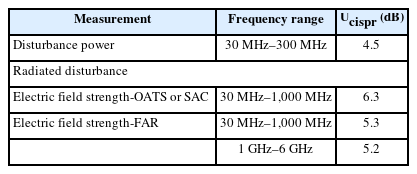
In Table 8, the frequency range conditions for radiated disturbance measurements (at an OATS, in a SAC, or in a FAR) match exactly those in our study. Here, the Ucispr values indicate the total uncertainty of the entire radiated disturbance measurement system. These values are used to demonstrate that the AF uncertainties within our study are acceptable. Considering the Ucispr values specified as 6.3 dB and 5.3 dB for these measurements, we can conclude that antennas calibrated with an uncertainty of 1.89 dB in our study can be easily used for these measurements in such a way that there is enough room for the uncertainties of other components of the measurement system.
As we highlighted earlier in this section, for the biconical antenna, the calibration with SSM-KA presents a curve similar to that with SSM-3A, while for the log-periodic antenna, we observe a small offset between the results of the two methods. Moreover, the maximum differences between the results of the two methods for both the biconical and log-periodic antennas almost fall within the measurement uncertainty of the known antenna method. As for the calibration process, SSM-KA shortens the experiment time by around 66% compared to SSM-3A.
In summary, considering the usage area, the calibration of EMC antennas can be performed by applying the SSM-KA method even in non-ideal test sites, such as the narrow one used in our study. This will have key advantages, such as practicality, fast implementation, and cost effectiveness. However, the experimenter should be careful in using a known antenna with low uncertainty, as this is the dominant contributor to the overall calibration uncertainty.
2. Comparative Results of SSM-3A and SSM-IA
As an application of SSM-IA, we measured the AFs of the R&S precision half-wave dipole sets listed in Table 4 (HZ-12, HZ-13) in our study. In the measurement process, the antenna height scan was limited to 1–3.5 m because of mechanical conditions/restrictions (vibration, mechanical stress, and bending). The comparison of the measured AFs, AFMEAS, and the values specified in the manufacturer’s manual, AFMANU, is presented in Table 9 and Fig. 6. The AFMANU values in Table 9 are obtained by adding the correction values in the manufacturer’s manual regarding the height of the antenna (R&S) [20]. As can be seen from Table 9, the difference between the measured AF and the values provided by the manufacturer (ΔAF = AFMEAS – AFMANU) is maximum at 40 MHz with 2.02 dB and drops significantly above 50 MHz. As stated in Section II.3, the antenna set HZ-13 was used for the 300 MHz–1,000 MHz frequency range; with this antenna pair, we therefore have a maximum difference of 1.36 dB at 700 MHz. At this point, we make our comments similar to those in the SSM-KA case. That is, the values should be evaluated depending on the intended use of the antenna, and in practice, these values are easily acceptable in many applications related to EMC measurements.

Measurement results and the manufacturer’s data for dipole sets
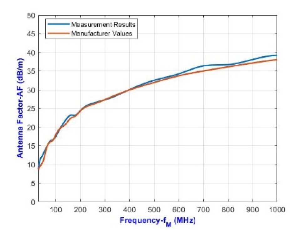
Comparison between the SSM (identical) and the manufacturer values for the dipole antennas.
Again, similar to SSM-KA, the calibration time with SSM-IA is reduced to approximately one-third compared with that with SSM-3A.
IV. Conclusion
This study explores the application possibilities of the SSM sub-cases of ANSI C63.5-2006 for EMC antenna calibrations in non-ideal conditions in terms of site dimensions. The study, which primarily aims to shorten the calibration time, is the next step in the work of [4], in which the method applied is SSM-3A.
In this context, the sub-cases SSM-KA and SSM-IA are discussed first, and then biconical and log-periodic antennas and dipole sets are calibrated accordingly in the frequency range of 30 MHz–1 GHz. The calibrations are performed at the OATS of the Turkish Standard Institution. This is a relatively narrow site, which was also used for the study in [4] and is beneficial for the EMC testing of products.
The importance of this study stands out in the following points:
Electromagnetic compatibility antenna calibrations are crucial, as these antennas are used for EMC tests of almost all electrical/electronic devices.
All around the world, there are test sites similar to that used in our study, but they are not ideal in terms of their dimensions. Nevertheless, they can still be used for antenna calibrations.
Calibration takes too long in accordance with the classic SSM-3A, so experimenters attempt to shorten the calibration process in order to save time and money.
We take advantage of SSM sub-cases that only need one site attenuation measurement.
In our study, we calculated the AFs of biconical and log-periodic antennas using the SSM-KA application; for the known antennas, we had calibration certificates from the reference institute, TUBITAK-UME. For the application of SMM-IA, we calibrated a half-wave dipole set and compared the results with those provided by the manufacturer (R&S).
The results obtained by applying SSM-KA on biconical and log-periodic antennas show good agreement with the values obtained by applying SMM-3A; the differences observed remain within practically acceptable limits. Our basis for this interpretation is the values allowed for EMC tests in the standards. To decide on the possibility of using antennas in EMC tests, we must consider the uncertainty limits allowed for the tests. In this context, we refer to the standard CISPR 16-4-2 in which these limits are defined. Considering these limit values, we conclude that the uncertainty in the measurement of AFs with SSM-KA is quite reasonable in our study. We note, however, that the dominant parameter in the uncertainty budget is the accuracy of the AF of the known antenna. Therefore, further improvements in overall uncertainty can be achieved by using a known antenna with higher accuracy/lower uncertainty.
Similar inferences also apply to the situation regarding SSM-IA implementation. The calibration results of the precision half-wave dipole sets, which are considered identical antennas, show good agreement with the manufacturers’ data. Again, we note that the conditions in the standards must be considered when deciding on the use of antennas in the relevant EMC tests. As for the solution to reduce the calibration time, the calibration process for both sub-cases requires about a third of the time as with SSM-3A.
In summary, in this study, we clarify that EMC antennas can be calibrated using SSM-KA and SSM-IA even in non-ideal test sites; in particular, it is the usage area conditions of these antennas that we need to focus on in terms of meeting the measurement uncertainty limits specified in the standards. Apart from the practicality of this approach, it helps economize by shortening the processing time while enabling the use of non-ideal test sites scattered across the world.
Acknowledgments
The authors express their sincere thanks to the Turkish Standards Institute for its unwavering support in the conduct of the experiments.
This study is an offshoot of the M.Sc. thesis written by the first author and supervised by the second author.
References
Biography

İlkcan Coşkun received his B.S. degree in mechatronics engineering from Kocaeli University and his M.S. degree in mechatronics engineering from Istanbul Technical University. In 2011, he joined the Ministry of Energy and Natural Resources in Ankara, Türkiye as a mechatronics engineer. From 2011 to 2017, he was with the Turkish Standard Institution Test and Calibration Center in Gebze, Türkiye, where he was a test/calibration engineer and the head of the electrical calibration laboratory. From 2017 to 2020, he was a researcher at TUBITAK UME (National Metrology Institute) in Gebze, Türkiye. He started to work as a functional safety engineer in the machinery department of ROSAS Center Fribourg in Switzerland in 2020, and today he continues as the head of the functional safety (machinery, automotive, railway, and aviation) department and test laboratory expert. His research interests include metrology (electrical, EMC, antennas, acoustic, vibration, and gravity), functional safety and cybersecurity, robotics, control, and automation systems.

Serhat İkizoğlu graduated from Istanbul Technical University (ITU)-Control and Computer Engineering. He received his Ph.D. degree from the same institution in 1992. He is currently an associate professor at ITU-Control and Automation Engineering Department. His areas of interest are measurement, instrumentation, control, and mechatronics.