Sidelobe Suppression Beamforming Using Tapered Amplitude Distribution for a Microwave Power Transfer System with a Planar Array Antenna

Article information

Abstract

I. Introduction

Microwave power transfer (MPT) is attracting attention for use in Internet of Things (IoT) and medical devices [1, 2] because it has the potential to transmit power over long distances, irrespective of the receiver’s (Rx) location. However, it also has the disadvantage of low efficiency due to path loss. To overcome this drawback, the transmitter (Tx) configures a massive array antenna and increases the magnitude of the radiated signal per channel. Unfortunately, this approach intensifies the sidelobe, which can adversely affect the surrounding electronics, as well as human beings; therefore, it is necessary to lower the sidelobe level (SLL) while maintaining the magnitude of the main lobe.

Several studies have been conducted on high-efficiency MPT, such as retro-reflective beamforming [3, 4]. This technique, which has been investigated for radar applications, transfers power efficiently by tracking the location of the Rx through a pilot signal and transmitting power in the same direction. Other studies on MPT have used look-up tables (LUTs) [5]. In this method, phase values for an array antenna that can transmit power optimally in the direction of the designated Rx antenna are stored in an LUT, with the beamforming directed toward the located Rx antenna. Although [3–5] achieved high efficiency under ideal conditions, they did not consider lowering the SLL; hence, MPT studies aiming to reduce SLL are underway [6–9].

A few researchers have applied various techniques for the non-uniform distribution of the magnitude of signals from array antennas; for example, [6] studied this for the application of MPT to drones. In their simulation, the researchers suppressed the SLL to −17.7 dB by applying a Gaussian function to the amplitude distribution of a 1 × 14 Tx array antenna at 5.8 GHz. In [7], the results for uniform amplitude distribution were compared to those for applying the Kaiser function to the amplitude distribution of an array antenna. The researchers verified through simulation that their technique reduced the SLL to −12.8 dB at 9.5 GHz. In [8], the Taylor function was applied to the feeding network of an array antenna. The researchers fabricated a 1 × 8 array antenna at 28 GHz and confirmed the reduction of SLL to −15.2 dB. Study [9] matched the weighting coefficient of the Chebyshev function to the feeding line impedance of an antenna.

The researchers designed a 1 × 5 array antenna at 9.3 GHz and verified the suppression of the SLL to −17.4 dB. However, the elements fabricated in these studies could only form one beam pattern for a fixed SLL. Different elements may be needed to achieve a minimum SLL for different beam directions. To overcome this drawback, we propose an adaptive beamforming system with sidelobe suppression that can actively form the desired beam. This paper presents a method for lowering SLL by adjusting the amplitude distribution of a two-dimensional planar array antenna (PAA). The phase distribution of a signal applied to an array antenna determines the direction of the main beam, and the amplitude distribution determines the SLL, main beamwidth, and nulls [10]; therefore, to reduce SLL, the amplitude of the array antenna must be distributed non-uniformly. This study proposes a method for obtaining an amplitude distribution matrix with the weight of each antenna as an element in an M × N PAA. This M × N matrix is derived as the product of the amplitude distribution vectors of two linear array antennas (LAAs) constituting the PAA. To lower the SLL while maintaining the total transmission power, we increased the amplitude of the signal applied to the central element of the array antenna and lowered the amplitude of the signal applied to the side element using the tapered amplitude distribution method [10]. Although this method reduces the sidelobe of the beam pattern, it weakens directivity owing to the widening of the beamwidth; therefore, we used the Chebyshev tapered amplitude distribution method, which is efficient and possesses the strongest directivity among distribution methods with the same maximum SLL [11]. Moreover, by limiting all sidelobes to the same level, we minimized the RF radiation power in all directions, except for the main lobe.

To verify the validity of the proposed method, we designed a digital beamforming system with a 4 × 4 Tx array and an Rx operating at 5.8 GHz. The Tx of the digital beamforming system was an adaptive device capable of generating signals with the desired phase and amplitude. Furthermore, for MPT, the Tx consisted of a digital Tx stage for RF signal generation and a power amplification (PA) stage. The magnitude of the signal from each channel of the Tx had a least significant bit (LSB) of 0.2 dB, and the phase had an LSB of 0.36°. The maximum output power per channel was 1 W. We conducted the measurements in the far field and verified the performance using the received power.

The remainder of this paper is organized as follows. Section II describes the sidelobe suppression method for the PAA. Section III explains the design, implementation, and simulation of the digital beamforming system for verification. Section IV conducts the experiments and discusses system performance. Finally, Section V presents the study’s conclusions.

II. Sidelobe Suppression Beamforming

Fig. 1 shows a schematic diagram illustrating the relationship between sidelobe and directivity during beamforming. It depicts steering of the main beam in the direction for received power and sidelobe suppression in the direction of the person to reduce power. As mentioned in the previous section, the sidelobe can be altered by manipulating the amplitude distribution of the array antenna, but a nonuniform amplitude distribution can widen the main lobe’s beamwidth [10], weakening the directivity of the array antenna. Directivity is the yardstick for power transmission in the intended direction; therefore, the SLL must be reduced as much as possible, and an amplitude distribution applied with high directivity. To this end, studies frequently use a tapered amplitude distribution to increase the amplitude of the central element antenna and decrease that of the side element antenna. The Chebyshev taper has the narrowest main lobe beamwidth, given a limited SLL [11]; therefore, we applied the Chebyshev taper to the amplitude distribution through an array factor (AF) of far-field approximation.

Fig. 1

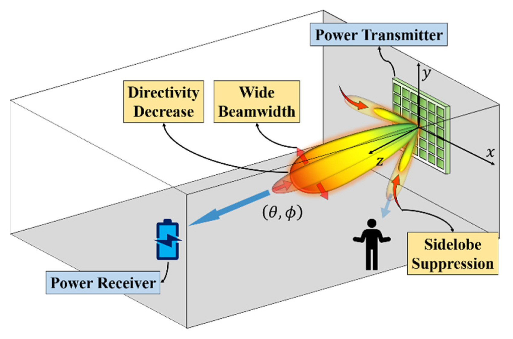
Sidelobe suppression beamforming considering directivity and beamwidth.

Fig. 2 depicts the structure of the PAA. As shown in Fig. 2, the PAA consists of two intersecting LAAs, and AF is equal to the product of the AFs of the two LAAs. The AFs of the two LAAs are as follows [10]:

Fig. 2

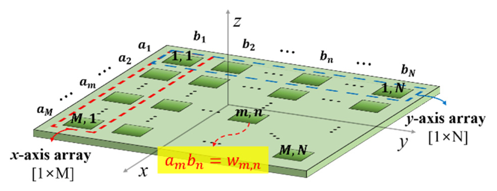
Geometry structure of the planar array antenna.

where a_m and b_n are the amplitude distributions of the x- and y-axis LAAs, M and N are the numbers of x-axis and y-axis array elements, d_x and d_y are the spacings between the elements of the x-axis and y-axis LAAs, and ψ_x and ψ_y are the phases of the x-axis and y-axis LAAs, respectively. k is the wave number, θ is the elevation angle, and φ is the azimuth angle. The amplitude distributions of the two axes, a_m and b_n, can be expressed as 1 × M and 1 × N vectors, respectively,

Furthermore, the AF of the PAA can be expressed by the product of Eqs. (1) and (2), as follows:

where w_m,n is the product of a_m and b_n. An M × N matrix with w_m,n, which is the amplitude distribution of the PAA, can then be expressed as follows:

To obtain Eq. (6), we analyzed the AFs of the LAA for the two axes. Since the phase and amplitude distributions are independent of each other in this process of obtaining the amplitude distribution, the phase (ψ_x and ψ_y) that determines the beam direction can be considered a constant; therefore, in Eq. (1), the AF of the x-axis LAA is a series of exponential functions that can be expressed as follows:

where ^{z = e j(kd_x sinθ cosφ +ψ _x)}. Eq. (7) is the same as the (M – 1)^th order equation, and can therefore be rewritten as

Because Eq. (8) is a polynomial of the degree (M – 1) equation, it can be expressed as a product of (M – 1) linear terms, as follows:

where z_i are the roots in the AF, β_i are the null directions, and i ranges from 1 to M – 1; hence, if the null directions are known, the roots of the AF can be found, and the AF expressed as the product of linear terms can be completed. The AF equation, which is the product of a linear term, is developed in polynomial form, and the coefficients of each term are mapped to the amplitude coefficients of the array antenna; hence, it describes the process for finding the null directions by mapping the Chebyshev polynomial [11] using the array factor. To this end, the difference in magnitude between the main lobe and the sidelobe is defined as follows:

where (θ_ML, φ_ML) is the main lobe direction and (θ_SL, φ_SL) is the sidelobe direction. We then derived the null directions (β_i) using the following equations:

and

This process is explained in detail in [12].

To determine the roots of the AF, null directions obtained through Eq. (12) were assigned to Eq. (10), and Eq. (9) was expanded as follows:

where w_xp is the weight of the p^th order term, and p ranges from 1 to M – 1. If a_M is a coefficient that determines the overall magnitude of the amplitude distribution, then the coefficient of each order (w_xp) can be expressed as a ratio; therefore, the amplitude distribution vector (1 × M) can be expressed as follows:

Applying Eqs. (7)–(14) to the y-axis LAA yields the following vector:

where w_yq is the weight of q^th order term, and q ranges from 1 to N – 1.

The coefficients of the linear vector in Eqs. (15) and (16) are the same as those of the Chebyshev taper, gradually increasing from the side element of the vector to the central element; hence, if Eqs. (15) and (16) are applied as weights of the array antenna, the radiated power from the side element antenna is low, and the radiated power from the central element antenna is high. This technique is often used to determine the weights in array antennas to form low sidelobes [9]. In this study, we need to know the amplitude distribution to be applied to the PAA; therefore, W, which is the Chebyshev tapered amplitude distribution for the M × N PAA, could be obtained through Eq. (6). This process ends by mapping the elements of W to the amplitude weights of each element of the PAA, allowing the realization of beamforming with an expected SLL. Fig. 3 illustrates the process flowchart for obtaining the Chebyshev tapered amplitude distribution for sidelobe suppression beamforming.

Fig. 3

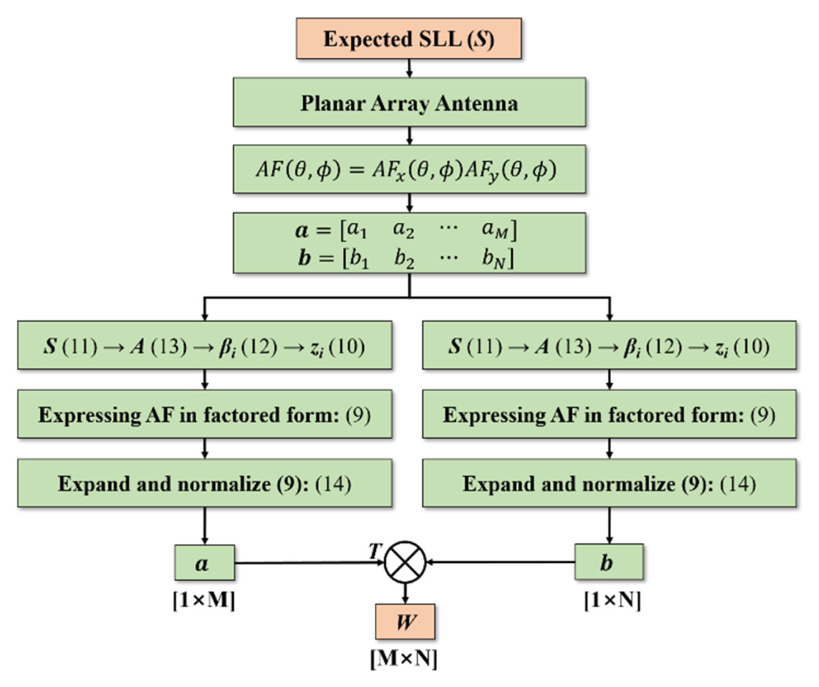
Flowchart of the process for finding the amplitude distribution of the PAA for sidelobe suppression beamforming.

III. System Design and Implementation

1. System Design

To verify the proposed sidelobe suppression scheme, we designed a digital beamforming system with a Tx array and an Rx operating at 5.8 GHz. Fig. 4 shows a block diagram of the system.

Fig. 4

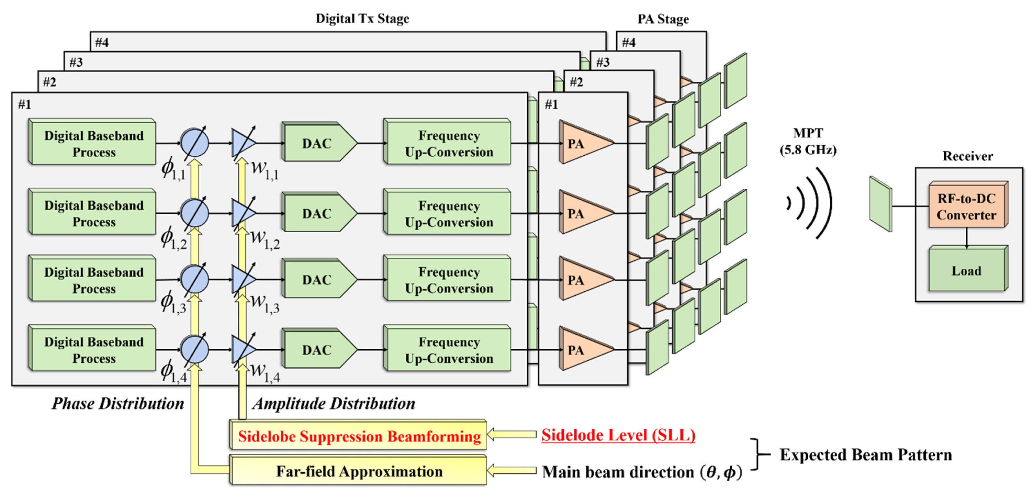
Block diagram of the digital beamforming system for MPT.

The Tx is a 4 × 4 array with 16 channels, a digital Tx stage, and a PA stage. The digital Tx stage generates an in-phase and quadrature (I/Q) signal, which is a baseband signal, and converts it to an analog signal through a digital-to-analog converter. We adjusted the I/Q signal using the sidelobe suppression beamforming method described in the previous section based on an LSB gain of 0.2 dB and an LSB phase of 0.36°. The analog baseband signal is converted into an RF signal through frequency upconversion and output. The RF signal is then applied to the PA stage of the MPT, and the signal is amplified. The PA stage uses a PA with a power gain of 32 dB and a P1dB of 33 dBm. The amplified RF signal radiates from a channel via a single antenna with a directivity of 9.3 dBi.

The Rx is composed of a single antenna, an RF-to-DC converter, and a load. The RF signal applied to the antenna is rectified to a DC signal by the RF-to-DC converter circuit. The Rx antenna is the same as a single Tx antenna with a directivity of 9.3 dBi.

Fig. 5 illustrates the antenna structure used in the digital beamforming system. The single antenna comprises a 2 × 2 sub-array with a single input port to increase the gain, as shown in Fig. 5. The feeding lines reaching each sub-antenna are designed identically, so that an in-phase signal is applied to or radiated from the sub-antenna. The substrate is made of a 0.8-mm-thick RF-35 laminate with a dielectric constant of 3.5 and a loss tangent of 0.002. It has a reflection coefficient of approximately −30 dB at 5.8 GHz, and it forms a vertically polarized RF signal.

Fig. 5

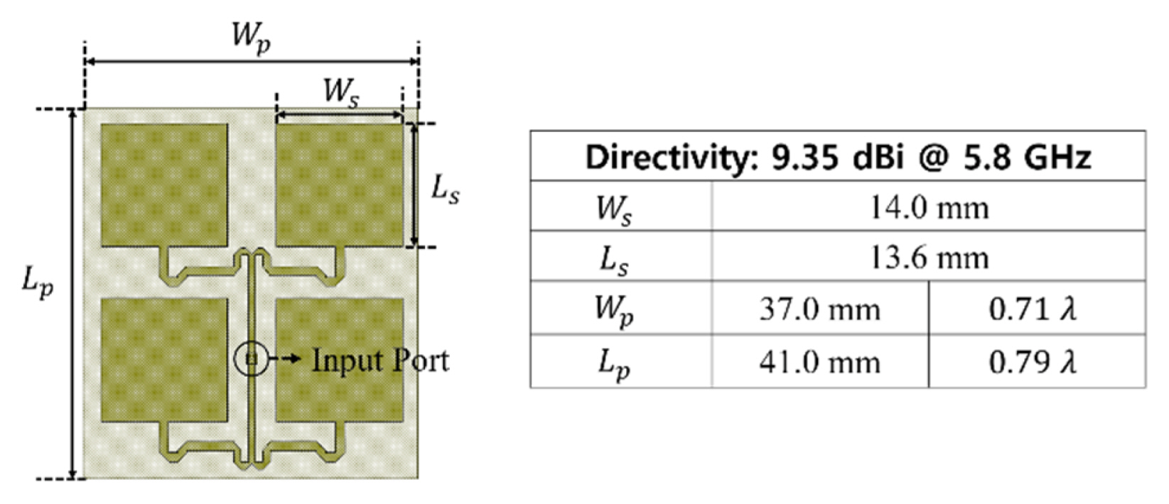
Structure of the single antenna with 2 × 2 sub-array.

Furthermore, the single antenna has a directivity of 9.3 dBi, and a 4 × 4 uniform array has 20.9 dBi. Fig. 6 shows the beam patterns simulated using AWR Microwave Office for the zx and zy planes, respectively.

Fig. 6

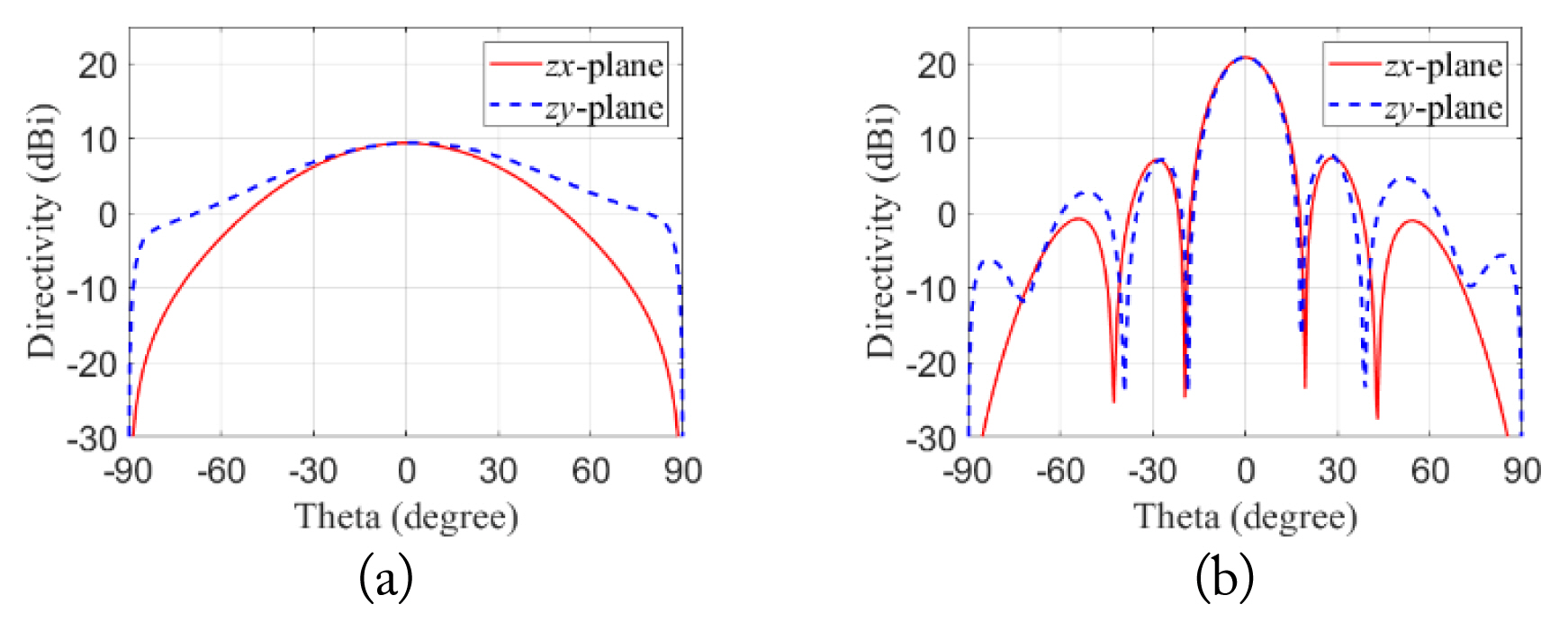
Simulated beam patterns: (a) single antenna and (b) array antenna.

2. Simulation

To verify the proposed sidelobe suppression method based on the designed digital beamforming system, we simulated the method. To incorporate the trade-off between the sidelobe and the directivity mentioned in Section II into the simulation, we had to analyze the mathematical relationship between the two. The tapered amplitude distribution of the LAA can be expressed as the efficiency in terms of directivity, as follows [12]:

(17) nT=DtaperDuniform=|∑m=1Lwm|2∑n=1L∑m=1Lsinc [(n-m) kd]L2∑n=1L∑m=1Lwnwm*sinc [(n-m) kd]

where D_taper is the directivity of the tapered array, D_uniform is the directivity of the uniform array, w_m is the amplitude distribution, d is the distance between elements, and L is the number of antenna elements. The amplitude distribution for the beam pattern with the expected SLL can be obtained using the scheme proposed in Section II. By applying the obtained amplitude distribution, the formed beam can be expressed as the efficiency of directivity. Fig. 7 shows the taper efficiency and normalized amplitude weights for array antennas with different antenna spacings on the x and y axes, as explained in the previous subsection (Section III-1).

Fig. 7

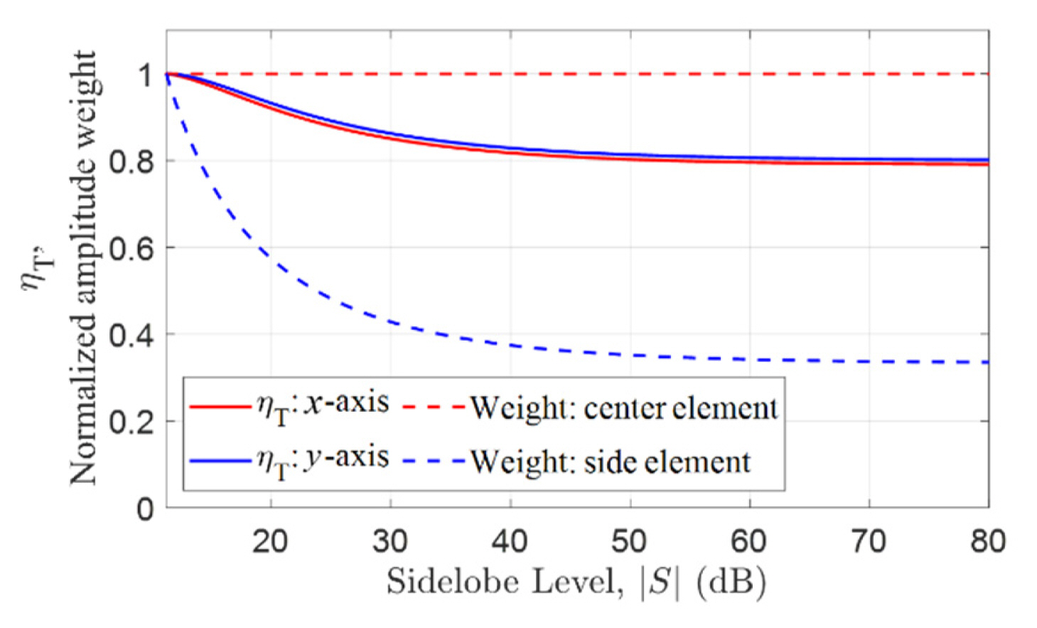
Taper efficiency and normalized amplitude weight.

As shown in Fig. 7, the taper efficiency (η_T) and the normalized amplitude of the central and side elements of the array antenna were presented according to S, which is the SLL. As S increases, the taper efficiency is saturated at a specific value, and the amplitude deviation of the central and side elements is also saturated. Therefore, we studied three cases: one for the uniform amplitude distribution (W₁), another for a taper efficiency of 0.9 (W₂), and the last for the moment of entering the region within 5% of the saturation section of the efficiency curve (W₃). Table 1 lists the SLL, amplitude distribution matrix (a, b) and taper efficiency (η_T) for each case. Fig. 8 shows the directivity when the amplitude distributions for each case were applied to the designed array antenna.

Table 1

Parameters of three amplitude distributions

Fig. 8

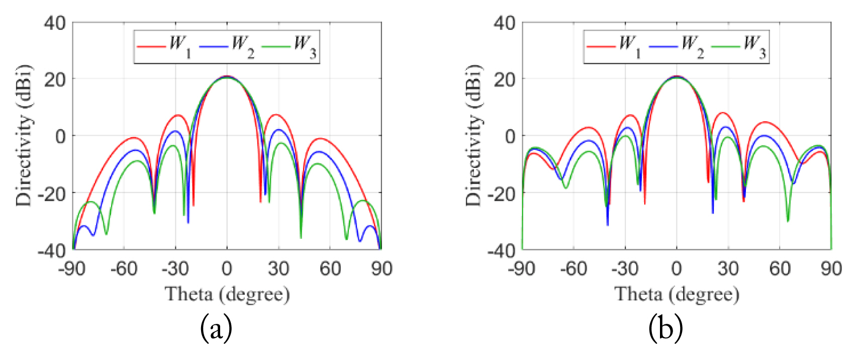
Simulated array antenna directivity of three amplitude distributions: (a) zx-plane and (b) zy-plane.

3. Implementation

Fig. 9 shows a photograph of the implemented Tx. Fig. 9(a) depicts a digital Tx stage composed of RF transceivers, microcomputers to drive them, and a clock distribution device. It also has a port for supplying power and a LAN port at the back, controlled via LabVIEW on an external PC. Fig. 9(b) depicts a PA stage with a 1 × 4 array PA consisting of four layers. The antenna was mounted directly on the output terminal. The digital Tx stage and PA stage were connected via coaxial cables. We used USRP B210 (a software-defined radio) as the RF transceiver and a CDA-2990 clock distribution device. We used Raspberry Pi 4B as the microcomputer, and QPA9501 as the PA.

Fig. 9

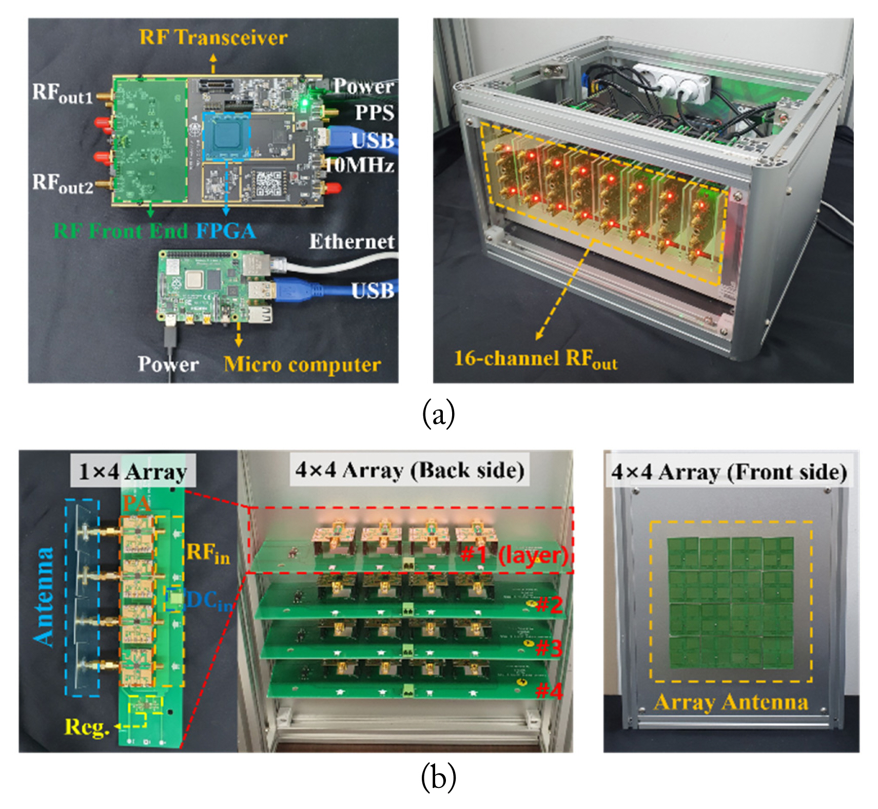
Implemented 4 × 4 Tx array: (a) digital Tx stage and (b) PA stage.

Fig. 10 shows a photograph of the Rx. A single antenna, directional coupler, and RF-to-DC converter circuit were connected via the RF adapter. The RF signal collected by the Rx antenna was applied to the input port of a directional coupler (Mini-Circuits ZGBDC35-93HP+) to simultaneously measure the RF and rectified DC power. The power was measured through the coupling port, and the output RF signal was rectified to a DC signal by the RF-to-DC converter connected directly to the output port. The RF-to-DC converter circuit had an embedded Schottky diode (BAT68-04W) with a voltage doubler. The power conversion efficiency of the circuit was 59.5%, which resulted from a rectified DC voltage of 6.5 V at an RF input power of 20 dBm and a load resistance of 600 Ω.

Fig. 10

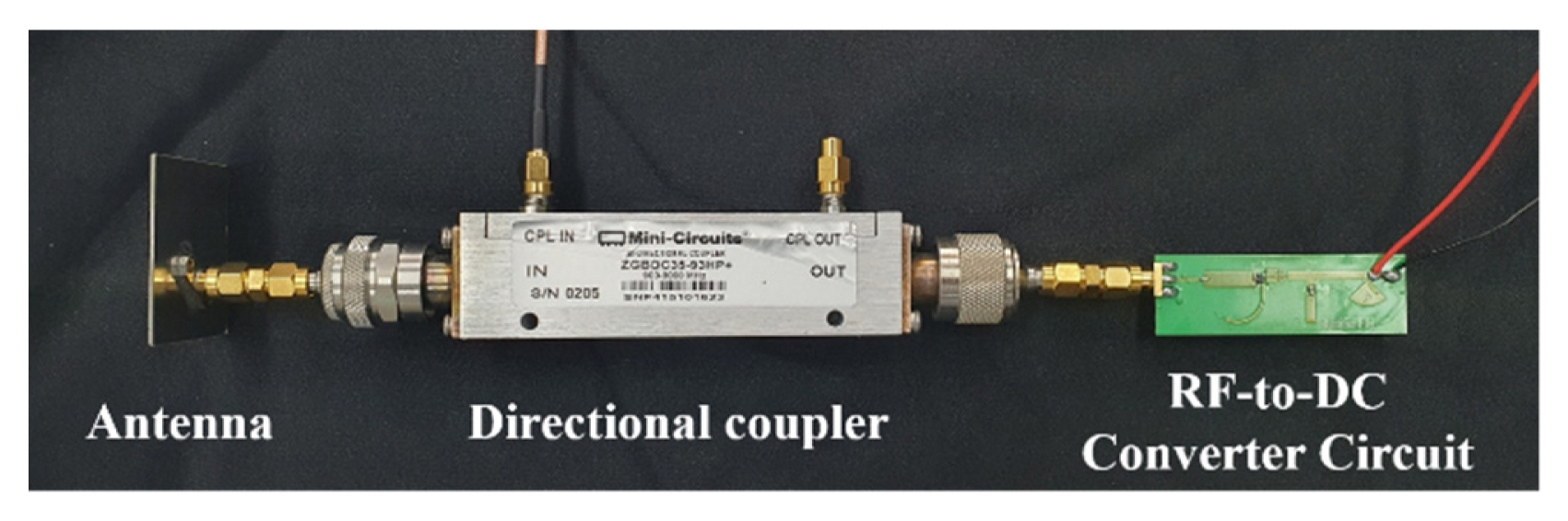
Implemented Rx.

The reflection coefficient (S₁₁) of the single antenna was −29.8 dB, measured with a network analyzer (Keysight P5007A), and the directivity of the 4 × 4 array antenna was determined as 21 dBi.

IV. Experimental Verification

Fig. 11 shows a photograph of the experimental setup for sidelobe suppression beamforming. The Tx was connected to the PC to control the beamforming system. The Rx was connected to a spectrum analyzer (Anritsu MS2713E) to measure the RF power and an electronic load (Keithley 2380-120-60) to measure the DC power. The gain of the transmitted RF signal was adjusted based on the three amplitude distributions obtained in Section III-2. The total RF power from the array antenna was fixed at 7.5 W (38.8 dBm) in all cases.

Fig. 11

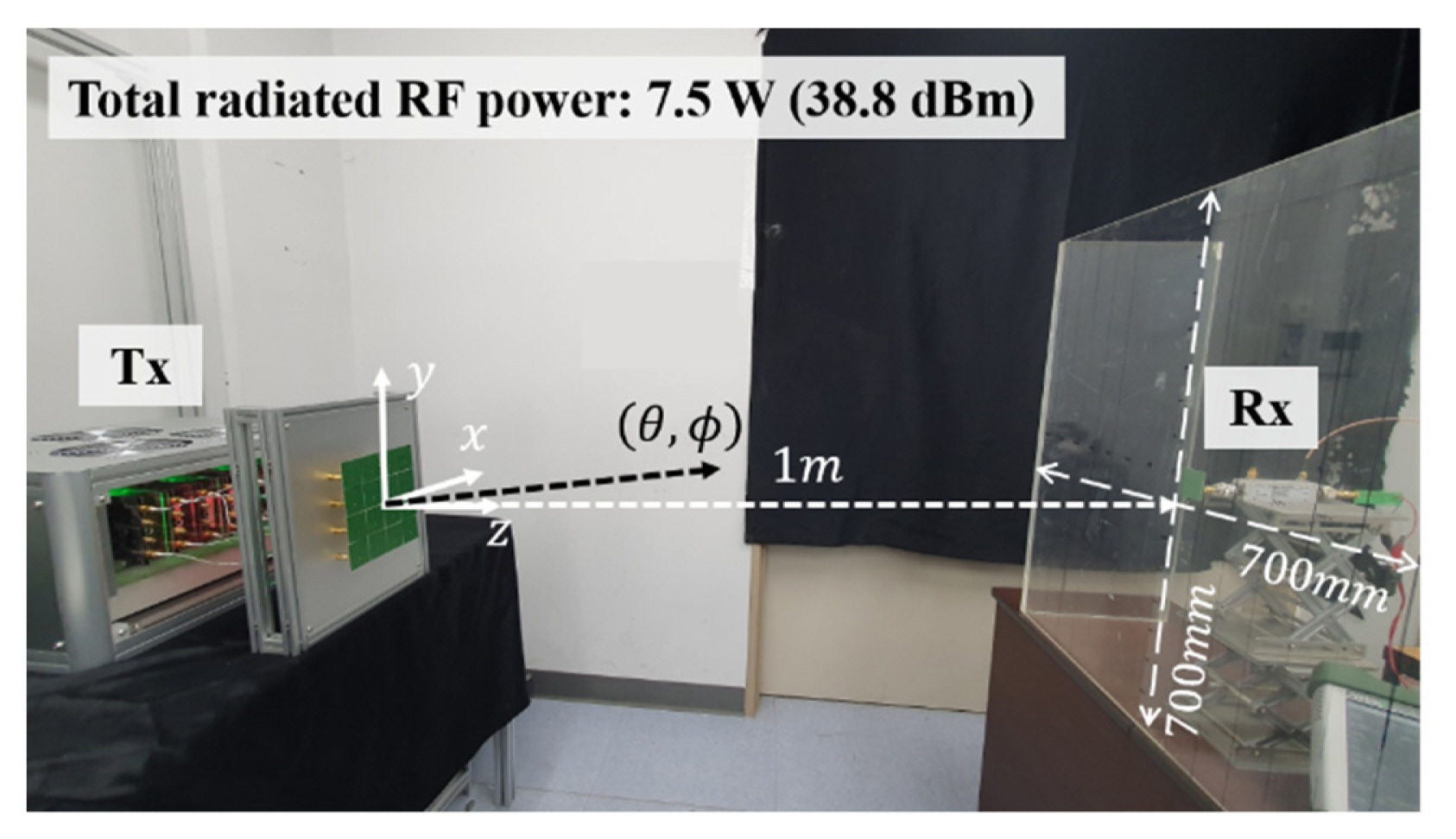
Experimental setup for sidelobe suppression beamforming.

Two experiments were conducted to verify the performance of the beamforming system. In the first, the radiation patterns of the zx and zy planes were measured. As shown in Fig. 11, this was based on the relative power by rotating the Tx array antenna in place while fixing the position of the Rx at the center. Fig. 12 illustrates the normalized radiation pattern plotted by measuring the received RF power from −90° to resemble that shown in Fig. 8, which resulted from the simulation. Compared with the SLL with W₁, which was a uniform distribution, the SLL while applying W₃ decreased by 7.5 dB from −11.6 dB to −19.1 dB on the zx plane and 4.4 dB from −11.5 dB to −15.9 dB on the zy plane. However, we confirmed that the received RF power at the central position (0°) decreased by only 0.6 dB, from 21.0 dBm to 20.4 dBm. Furthermore, we verified that the rectified DC power also decreased by only 9.3 mW, from 67.8 mW to 58.5 mW.

Fig. 12

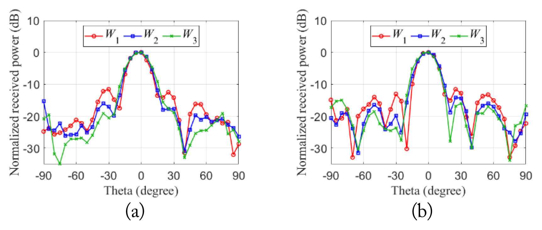
Measured radiation patterns of three amplitude distributions: (a) zx-plane, (b) zy-plane.

In the second experiment, we verified the performance of beamforming in specific directions. As depicted in Fig. 11, the received RF power of 15 × 15 points was measured on the plane (700 × 700 mm²) where the Rx could exist. The phase values for each channel of the main beam direction were adjusted by (5), giving the AF of the far field approximation. The main beam direction was set as (θ, φ), with the center of the Tx array antenna as the origin in spherical coordinate systems. The experiment was conducted for three main beam directions, when (θ, φ) was (0°, 0°), (20°, 135°), and (20°, 220°), respectively. Therefore, nine experiments in total were conducted for the three cases of amplitude distribution and three cases of phase distribution. Table 2 shows the distributions except for W₁ and (0°, 0°) where all the amplitudes and phases of the channels were identical. Fig. 13 shows a color map obtained by measuring the 15 × 15 points of normalized received RF power for the nine experiments. We confirmed that the region with the sidelobe had smaller power in W₂ and W₃ than in W₁. Additionally, we verified the widening of the main lobe with an increase in the area occupied by power in the direction of the main lobe. Table 3 summarizes the results of the second experiment, including the received RF power and SLL for the nine measurements. Furthermore, we calculated Δpower and ΔSLL (the differences between the received power and the SLL) from the uniform amplitude distribution (i.e., W₁). In (0°, 0°)—the case with central beamforming—received power was the same as in the first experiment, but the SLL decreased further. This occurred because the origin of the measured 15 × 15 points was 1 m away from the Tx, but the remaining points were at greater distances than 1 m, meaning that the received power was lower. Therefore, in the case of beamforming toward the center, we confirmed ΔSLL to be 9.3 dB at the maximum. In (20°, 135°)—the case with the second direction—ΔSLL and Δpower were 5.9 dB and 0.8 dB in W₃, respectively. Additionally, in (20°, 220°)—the case with the third direction—ΔSLL and Δpower were 6.8 dB and 0.5 dB in W₃, respectively. These results proved that the received power barely decreased and that the SLL decreased significantly.

Table 2

Amplitude and phase distributions for 4 × 4 array

Fig. 13

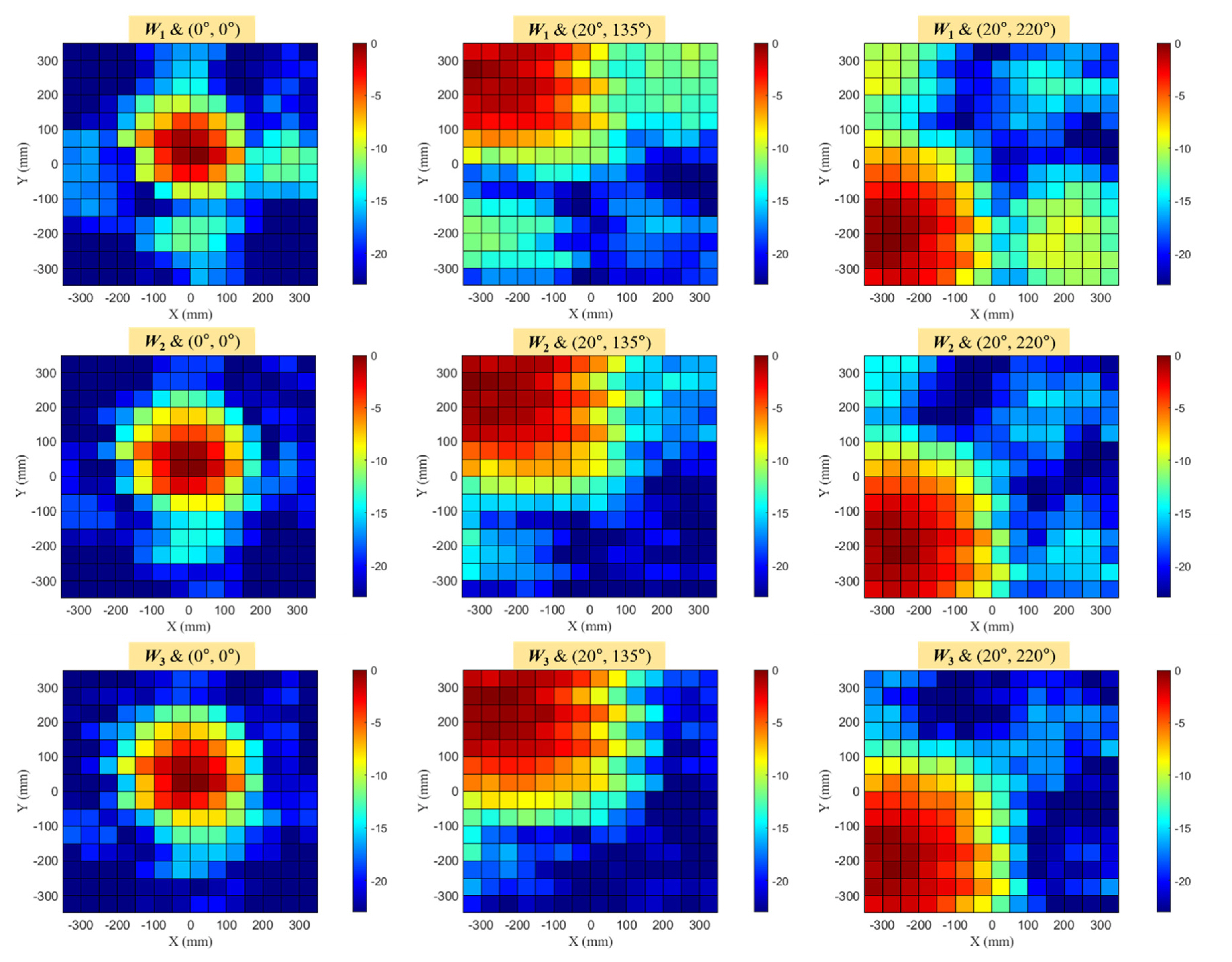
Color maps of normalized received RF power in the beamforming experiments for three amplitude and phase distributions.

Table 3

Results of beamforming experiments for three amplitude and phase distributions

The experimental results compared with other studies on MPT are listed in Table 4. As mentioned earlier, the comparison was based on the beam pattern of the zx plane in Fig. 12, which resulted from the first experiment. Studies [3–5] focused on the beamforming technique without considering lowering the sidelobe, and, in most cases, demonstrated high SLL. Additionally, [6–9] designed and manufactured a Tx device using a technique to lower the SLL, but different elements may be required to achieve a minimum SLL for other beam directions. The proposed sidelobe suppression beamforming system is suitable for safe wireless power transmission with high received power and low SLL.

Table 4

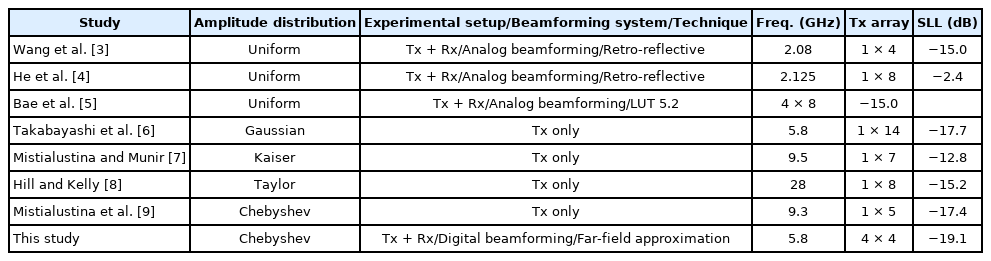
Comparison with other studies

V. Conclusion

This paper proposes a sidelobe suppression beamforming scheme for an MPT system with PAA. The technique applied to the proposed system involves controlling the magnitude of the signal transmitted from the array antenna. To apply this to a two-dimensional PAA, we described the procedure for obtaining the amplitude distribution matrix (M × N). Furthermore, to minimize decreased directivity due to the non-uniform amplitude distribution and to lower the SLL, we used the Chebyshev taper for the amplitude distribution.

To verify the proposed scheme, we implemented a digital beamforming system with a 4 × 4 Tx array and an Rx at 5.8 GHz. The radiation pattern results while adjusting the amplitude distribution confirmed that the SLL decreased by 7.5 dB to −19.1 dB on the zx plane, and by 4.4 dB to −15.9 dB on the zy plane, compared with uniform distribution. Furthermore, we verified that the received RF power was 20.4 dBm, even with sidelobe suppression. This amounted to a reduction of only 0.6 dB compared with the uniform distribution case. Through a color map, we demonstrated that the area occupied by the sidelobe decreased in the three-directional beamforming experiment. Moreover, compared with other studies, the proposed system has independent and flexible amplitude and phase control. Consequently, the adaptive beamforming system presented in this paper should be capable of delivering efficient and safe MPT by accurately forming a designed beam pattern.

Article information Continued

References

Biography
Inho Park received his B.Sc. degree in electronic engineering from Konkuk University, Seoul, South Korea, in 2021. He is currently pursuing his M.Sc. degree in electronic engineering at the same institute. His current research interests include wireless power transfer and digital RF systems.
Hyunchul Ku received his B.Sc. and M.Sc. degrees in electrical engineering from Seoul National University, Seoul, South Korea, in 1995 and 1997, respectively, and a Ph.D. in electrical and computer engineering from the Georgia Institute of Technology, Atlanta, GA, USA, in 2003. From 1997 to 1999, he worked at the Wireless Communication Research Center in KT, Seoul. From 2004 to 2005, he was employed at the Research and Development Laboratory, Mobile Communication Division, Samsung Electronics, Suwon, South Korea. Since 2005, he has worked as a professor at Konkuk University. His research interests include digital RF systems, RF power amplifiers, RF front-end design, and wireless power transfer systems.
Chulhun Seo received his B.Sc., M.Sc., and Ph.D. degrees from Seoul National University, Seoul, South Korea, in 1983, 1985, and 1993, respectively. From 1993 to 1995, he was employed by the Massachusetts Institute of Technology (MIT), Cambridge, MA, USA, as a technical staff member, and as a visiting professor from 1999 to 2001. From 1993 to 1997, he was employed by Soongsil University, Seoul, as an assistant professor, where he was also an associate professor from 1997 to 2004. Since 2004, he has been a professor of electronic engineering at Soongsil University. He was the IEEE MTT Korea chapter chairperson from 2011 to 2014. He is the president of the Korean Institute of Electromagnetic Engineering and Science (KIEES) and the dean of the Information and Telecommunications College at Soongsil University. He is the director of the Wireless Power Transfer Research Center, supported by the Korean Government’s Ministry of Trade, Industry, and Energy; the Metamaterials Research Center, supported by Basic Research Laboratories (BRL) through an NRF Grant funded by the Ministry of Science, ICT, and Future Planning (MSIP); and the Center for Intelligent Biomedical Wireless Power Transfer, supported by the National Research Foundation of Korea (NRF; grant funded by MSIP). His research interests include wireless technologies, RF power amplifiers, and wireless power transfer using metamaterials.