


I. Introduction
A coaxial waveguide is a fundamental transmission line to stably guide a light for optoelectronics [1ŌĆō3] or precisely measure the reflection coefficient and impedance up to millimeter-wave bands [4, 5]. Accurate evaluation of wave propagation through a practical coaxial waveguide is essential for quantifying measurement uncertainty occurring in microwave transmission [5]. Even in the visible spectrum, a nanocoax [3] is one of the promising structures for low-loss propagation composed of plasmonic and photonic modes, where the permittivity can be negative or complex to model real metals at optical frequency.
Since a practical coaxial line is inherently lossy owing to finite electrical conductivity, the TM wave (Ez ŌēĀ 0, Hz = 0) instead of the TEM wave (Ez = 0, Hz = 0) propagates and is gradually decreased in the z-direction. This behavior makes the dispersion analysis of the lossy coaxial waveguide more involved. Therefore, it is of great importance to derive and formulate an exact and rigorous dispersion relation of the lossy coaxial waveguide, which can be modeled as a multilayered dielectric coaxial waveguide [1, 6ŌĆō8]. A dielectric coaxial waveguide was analyzed using the boundary conditions of an open region [6] and an infinitely lossy outer conductor [7, 8]. In the following sections, we apply a standard mode-matching technique [9] for analyzing a dielectric coaxial waveguide surrounded by the perfect electric conductor (PEC) boundary. A newly-derived rigorous dispersion relation is used to determine precise complex propagation constants for the hybrid, TM, and TE modes in microwave and optical spectra, where we use DavidenkoŌĆÖs method [10, 11] for searching complex roots.
Using the conductor condition or high permittivity approximation, we obtained simplified but accurate dispersion equations useful for characterizing the transmission behaviors of the lossy coaxial waveguide. This means that our rigorous dispersion equations can be utilized to generate the field distributions for the TM0p, TE0p, EHmp, and HEmp modes and formulate the scattering characteristics of canonical coaxial structures used in a coaxial calibration kit [5]. The quasi-TEM mode also yields a closed-form approximate solution for the TM01-mode complex propagation constant, which becomes identical to the propagation constant [5, 7] in the high electrical conductivity limit.
II. Mode-Matching Analysis
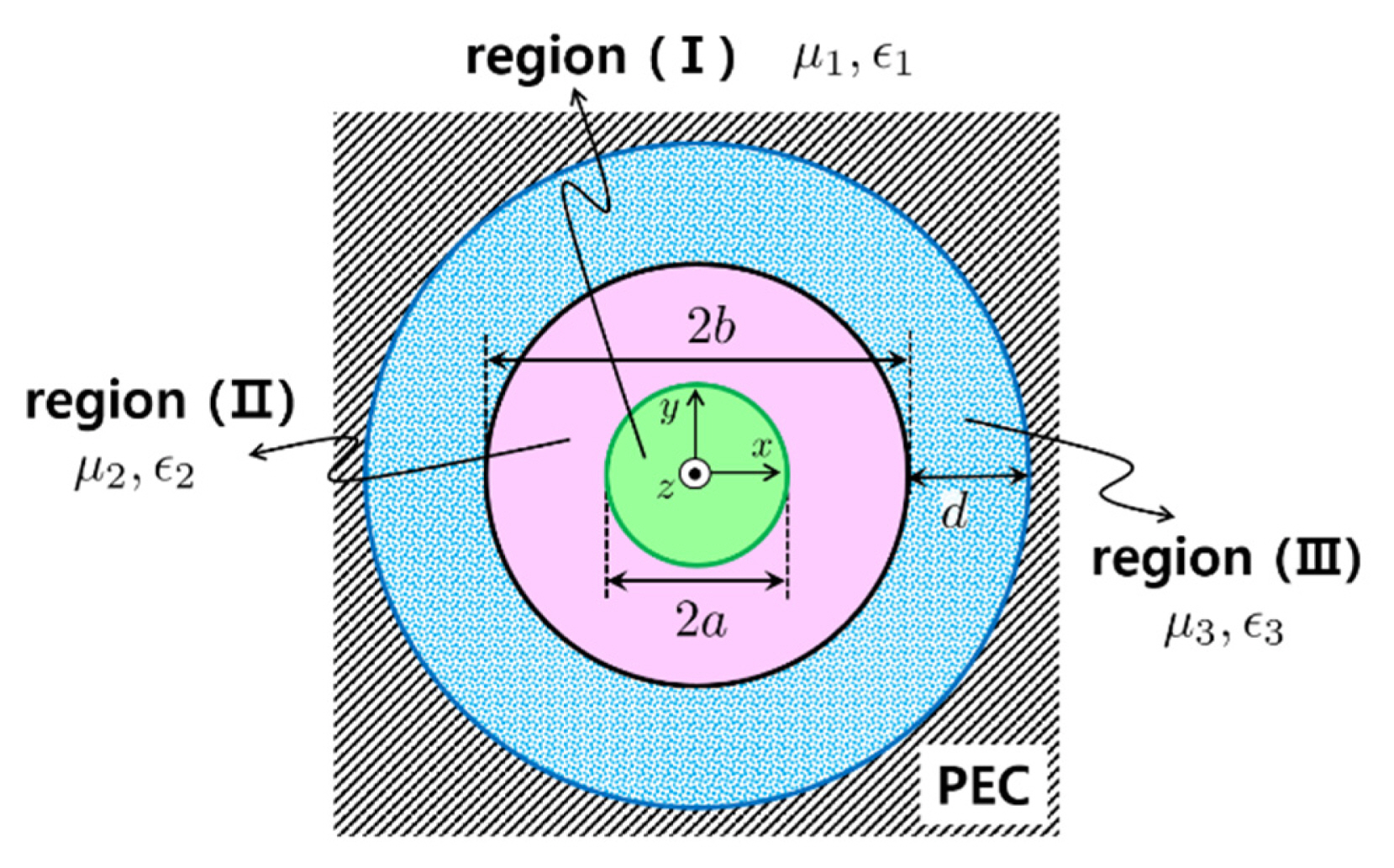
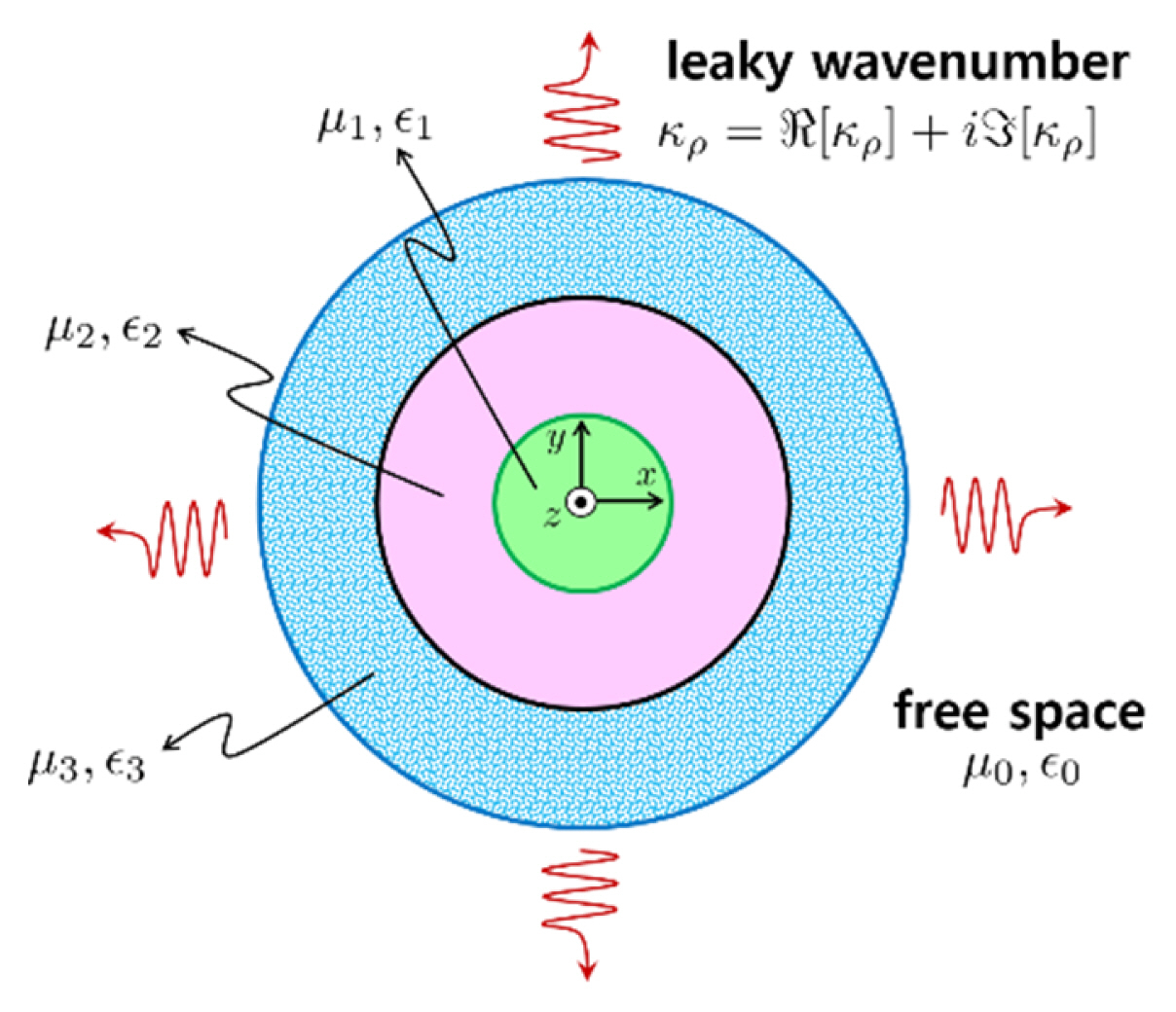
A lossy coaxial waveguide can be modeled using a multilayered dielectric coaxial waveguide [1, 6ŌĆō8] as shown in Fig. 1, where the medium constantsŌĆö╬Ą1, ╬Ą2, ╬Ą3 and ╬╝1, ╬╝2, ╬╝3ŌĆöcan be any complex number. We use and omit ei(╬▓zŌĆōŽēt) for the time convention, where ╬▓ is a complex propagation constant composed of phase (Ōä£[╬▓]) and attenuation (Ōäæ[╬▓]) constants. The interesting point of the geometry shown in Fig. 1 is that a dielectric coaxial waveguide [1, 6ŌĆō8] shown in Fig. 2 is entirely surrounded by the PEC boundary. It is known that unwanted multiple leaky modes [11] are inevitably generated in open magnetodielectric waveguides including dielectric coaxial structures [1, 6] with an open boundary as shown in Fig. 2. The existence of leaky phenomena caused by the open boundary makes a dispersion analysis of the dielectric coaxial waveguide much more involved. For instance, the dielectric coaxial waveguide shown in Fig. 2 should satisfy a leaky dispersion relation in an open region as
where
k 0 = Žē ╬╝ 0 ╔ø 0 Žü = x 2 + y 2
where the phase term of a guided wave is ei(╬║ŽüŽü+╬▓z). Eq. (2) indicates that the radial and longitudinal radiation conditions of ╬║Žü and ╬▓ cannot be satisfied at the same time, owing to the fact that the signs of the real or imaginary parts of ╬║Žü and ╬▓ are always different from each other. Contrary to the geometry shown in Fig. 2, the PEC boundary and lossy region (III) introduced in Fig. 1 enable us to block the leaky modes completely and model the conductor loss precisely. This is because the PEC boundary at Žü = b + d is imposed and ╬Ą3 can be complex, thus confirming there are no leaky modes and the waves are evanescent in region (III). Therefore, the field representations for regions (I) through (III) as shown in Fig. 1 are formulated using magnetic and electric vector potentials [9]:
where Am, Bm,
E m ( 1 ) , ( 2 ) , F m ( 1 ) , ( 2 ) Žü = x 2 + y 2 ╬║ n = k n 2 - ╬▓ 2 , ŌĆē k n = Žē ╬╝ n ╔ø n
and (┬Ę)ŌĆ▓ denotes differentiation for the entire argument; Jm(┬Ę) and Nm(┬Ę) are the mth order Bessel functions of the first and second kinds, respectively. Based on the standard mode-matching analysis [9], we enforce Ez-, EŽå-, Hz-, and HŽå-field continuities at Žü = a and b for the mth azimuthal mode. First, by multiplying the Ez- and Hz-field continuities at Žü = a by eŌłÆilŽå (l = 0, ┬▒1, ┬▒2, ┬Ę┬Ę┬Ę) and integrating over 0 Ōēż Žå Ōēż 2ŽĆ yields, respectively, we get:
where un = ╬║na,
Next, we apply and integrate the EŽå- and the HŽå-field continuities at Žü = a with eŌłÆilŽå to obtain the additional field-matching equations, respectively:
where
Z n TE = Žē ╬╝ n ╬▓ , ŌĆē Y n TM = Žē ╔ø n ╬▓ , ŌĆē ╔ø m ŌĆ▓ ( u ) = d d u ╔ø m ( u ) Žå m ŌĆ▓ ( u ) = d d u Žå m ( u ) E m ( 1 ) , ( 2 ) , F m ( 1 ) , ( 2 )
where vn=╬║nb. Combining and simplifying Eqs. (11), (12), and (15)ŌĆō(20), we obtained the mth hybrid-mode dispersion relation as
where |A| is the determinant of a matrix A and a system of simultaneous equations for
E m ( 1 ) , ( 2 ) , F m ( 1 ) , ( 2 )
(22)
The elements of ╬”m(╬▓) are defined by:
where
Therefore, a complex propagation constant ╬▓ can be determined by solving Eq. (21). When m = 0, the hybrid-mode dispersion relation shown in Eq. (21) can be divided into
(30)
Eq. (30) clearly proves that the TM and TE modes exist for m = 0, although the coaxial waveguide is filled with lossy dielectrics. Since Eq. (21) is applicable to a general coaxial waveguide of any ╬╝n and ╬Ąn, we can use Eq. (21) to analyze canonical waveguides, including the PEC circular and coaxial waveguides. For instance, when ╬╝n = ╬╝0 and ╬Ąn = ╬Ą0, the geometry shown in Fig. 1 becomes a PEC circular waveguide with a radius of b + d, and Eq. (21) is thus simplified to
III. Numerical Computations
We used DavidenkoŌĆÖs method [10, 11] to search a complex root ╬▓ by equating |╬”m(╬▓)| = 0 as shown in Eq. (21). DavidenkoŌĆÖs method in [11] uses the fourth-order RungeŌĆōKutta method and the NewtonŌĆōRaphson method in the complex domain, which is suitable for searching the complex propagation constant ╬▓. An iterative update equation for the next approximate solution ╬▓n+1 is given by
where ╬▓n is the current approximate value for ╬▓ and ╬ö╬▓n+1 is defined in [11, Eq. (10)]. The next differential step ╬ö╬▓n+1 is computed using ╬▓n, ╬ö╬▓n, and h, where ╬▓0 and ╬ö╬▓0 are the initial value and step for root searching, respectively, and h is a fixed step of the RungeŌĆōKutta method. As n increases very steeply, ╬▓n+1 stably converges to ╬▓ [10, 11]. We set h = 1 and ╬ö╬▓0 = ╬▓0/100 for all root-searching computations.
The TM01-mode dispersion results of the lossy coaxial waveguide are shown in Fig. 3 using m = 0 and f = 100 GHz, where the TM01 mode (m = 0) is a dominant quasi-TEM mode. We assume that regions (I) and (III) are filled with lossy conductors using
╔ø 1 = ╔ø 3 = ╔ø 0 ŌĆē ( 1 + i Žā Žē ╔ø 0 )
where Pn = ╬Ą2╬║n/╬Ąn╬║2,
Note that setting Um(v2) and
V m ŌĆ▓ ( v 2 )
when u ŌåÆ 0, N0(u) and
N 0 ŌĆ▓ ( u ) 2 ŽĆ lnŌĆē ( u 2 ) 2 ŽĆ u
Note that Eq. (38) is identical to [7, Eq. (37)] even though the boundary conditions for the outer conductors are different from each other. When ╬╝n = ╬╝0 and Žā Ōē½ 1, Eq. (38) becomes a complex propagation constant [5] obtained by the transmission line theory and penetration depth ╬┤s. Fig. 3 clearly indicates that the thickness (d) of an outer conductor hardly affects complex dispersion relations for Žā Ōēź 103 S/m and d Ōēź 0.2 mm Ōēł4╬┤s, where ╬┤s Ōēł 50 ╬╝m and Žā = 103 S/m. A comparison with [8] provides a favorable agreement when Žā Ōēź 103 S/m. This is because [8] assumes an infinite outer conductor (d ŌåÆ Ōł×) and the effects of the thick outer conductor are negligible for high electrical conductivity, where the outer conductor shown in Fig. 1 has finite thickness (d), which differs from [8]. As is also shown in Fig. 3, Eqs. (34) and (38) are practically good formulas in lieu of Eq. (21) for Žā Ōēź 103 S/m. When Žā approaches zero, Eq. (31) predicts that ╬▓ becomes that of a PEC circular waveguide denoted as ŌŚŗ in Fig. 3. The insets in Fig. 3 illustrate the normalized real and imaginary parts of the Ez-field distributions when Žā = 104 S/m and ╬▓ Ōēł 2161.77+65.96i rad/m. The real and imaginary Ez-fields of the TM01 mode are continuous across the boundaries at Žü = a and b, thus verifying that DavidenkoŌĆÖs method in Eq. (33) is effective for searching the complex root ╬▓ of a lossy coaxial waveguide. In addition, the magnitude of the Ez-fields is rapidly attenuated within lossy dielectrics in regions (I) and (III), and thus their field distributions illustrate the behaviors of the penetration depth very well.
Fig. 4 shows the dispersion behaviors of the TM01, TE01, and EH11 modes in the lossy coaxial waveguide versus microwave frequency. The TM01 mode has the lowest attenuation when compared with the TE01 and EH11 modes, thus indicating that the TM01 mode is a dominant mode irrespective of Žā. Applying Eq. (30) and the conductor condition (|╬Ą1| Ōē½ 1, |╬Ą3| Ōē½ 1) yields an approximate dispersion equation for the TE0p mode as
where Qn = ╬╝n╬║2/╬╝2╬║n. Similar to Eqs. (34) and (39), the dispersion relation Eq. (21) approximately reduces to
(40)
When Žā Ōēź 107 S/m, the magnitude of ╬Ą1 and ╬Ą3 becomes very high and thus the TE01- and EH11-mode ╬▓ computed by Eqs. (39) and (40) agree well with more precise solutions obtained by Eqs. (30) and (21), respectively. In Fig. 4, the attenuation constant (Ōäæ[╬▓]) of the EH11 mode rapidly decreases above fc Ōēł 135.9 GHz. Therefore, the TM01 and EH11 modes coexist and propagate along the lossy coaxial waveguide above fc. Considering Eq. (40), the cutoff frequency (fc) of the lossy EH11 mode can be approximately determined using
V 1 ŌĆ▓ ( v 2 ) Ōēł 0
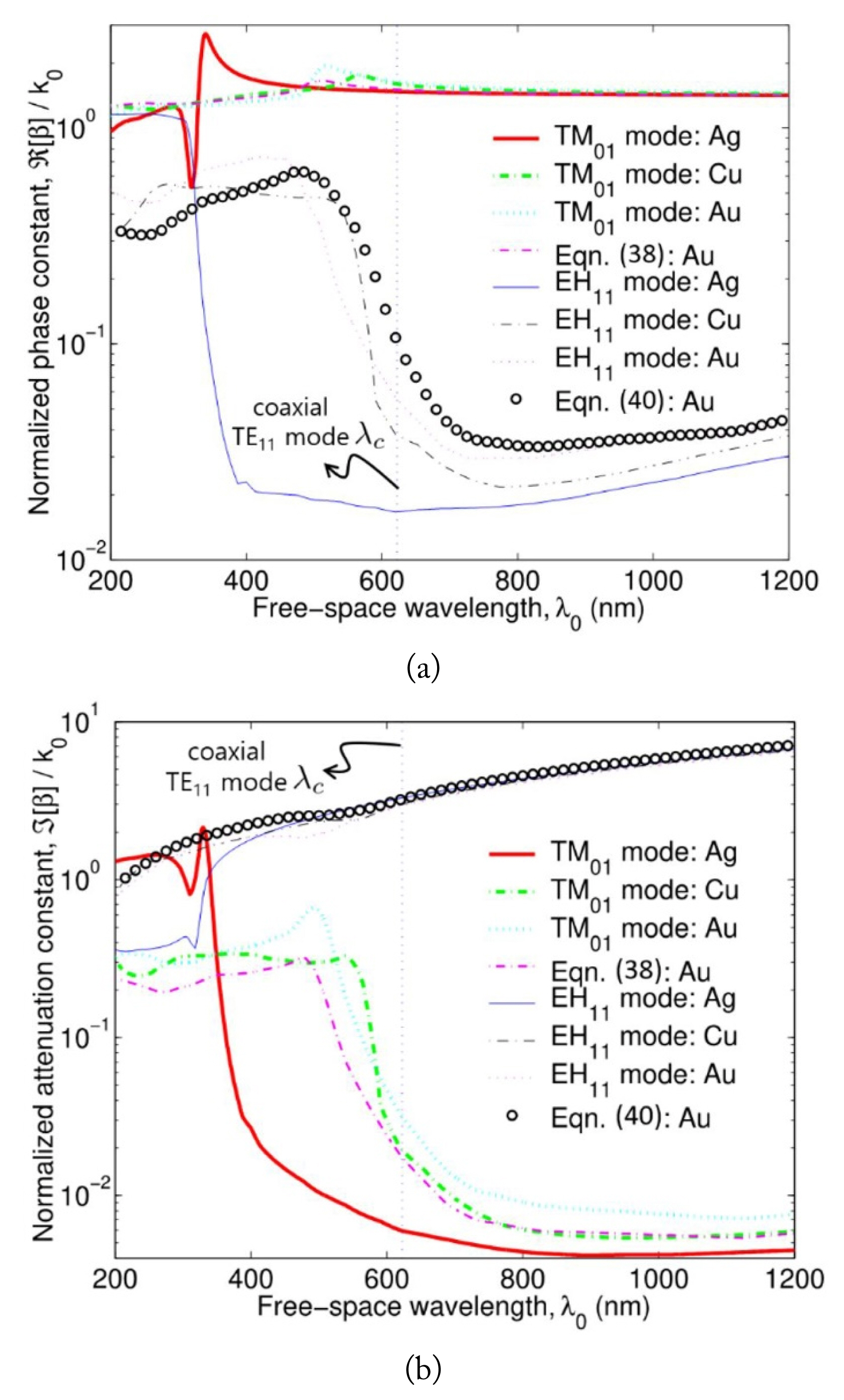
Fig. 5 illustrates the dispersion characteristics of the TM01 and EH11 modes within the visible spectrum. To theoretically obtain the dispersion relations of the lossy coaxial wave-guide composed of real metals, we use optical dielectric constants [12] of silver (Ag), copper (Cu), and gold (Au). In the visible spectrum, the real part of the metal permittivity is usually negative caused by plasma oscillation in the metal. Fig. 5 indicates that Eq. (38) is valid within the optical spectrum and the cutoff or transition wavelength (╬╗c) can be obtained by Eq. (40). As a result, our approximate solutions obtained from Eqs. (38) and (40) are useful for predicting the optical behaviors of the TM01 and EH11 modes in the nanoscale coaxial waveguide.
IV. Conclusion
Analytical hybrid-mode dispersion relations of the lossy coaxial waveguide are presented based on the mode-matching technique and the vector potential formulations. Precise phase and attenuation constants of the TM01, TE01, and EH11 modes have been numerically evaluated using the root-searching algorithm based on DavidenkoŌĆÖs method. Approximate but accurate dispersion equations for the TM0p, TE0p, EHmp, and HEmp modes are also proposed and agree well with more rigorous dispersion relations even for low electric conductivity or negative permittivity. Our dispersion solutions can be applied to the theoretical evaluation of a coaxial calibration kit or the analytical determination of light distribution within the optical coaxial waveguide.