Analysis of the Envelope Correlation Coefficient of MIMO Antennas Connected with Suspended Lines

Article information

Abstract

I. Introduction

As information communication technology has been selected as the core growth engine of the fourth industrial revolution, there is a growing interest in constructing a network infrastructure with low latency and high connectivity. Fifth generation (5G) mobile communication is the technology on which such a network environment is based and is being actively implemented in several tech-leading countries. One of the key technologies employed not only in 4G but also in 5G is the multiple-input multiple-output (MIMO) antenna. This technology dramatically increases the data transmission rate without increasing the bandwidth or transmitting power by arranging multiple antennas at the transmitting and receiving ends [1, 2]. In general, the performance of the MIMO antenna is strongly affected by the envelope correlation coefficient (ECC) between the antenna elements; a lower ECC offers the best performance [3]. The mutual coupling (MC) between the antennas significantly affects ECC. For example, the narrower the distance between the antenna elements, the stronger the mutual interference and the more fatal the effect on ECC and the overall MIMO system. To apply the MIMO antenna technology to a limited space (e.g., inside a cellphone), the MC and ECC problems must be solved simultaneously [4].

Many antenna structures and alignment techniques have been studied to solve this problem [5–10]. The most intuitive way to reduce the ECC of MIMO antennas is to increase space diversity or polarization diversity by widening the distance between the antenna elements or rotating the elements orthogonally to each other [5, 6]. However, this is not suitable for MIMO antennas implemented in a limited space. A defected ground structure (DGS) was proposed to reduce the ECC by changing the surface current distribution flowing on the ground plane [7, 8]. However, its use is limited because additional patterning on the ground is not preferred for the manufacturing viewpoint, and DGS patterns usually generate unwanted back lobes. Similarly, an electromagnetic band-gap (EBG) structure was proposed to reduce the ECC by suppressing surface waves on the ground plane [9, 10]. However, the EBG structure complicates the antenna structure, and it is not suitable when the antenna elements are closely placed.

Inserting a suspended line between antenna elements is one promising way to reduce the ECC. The suspended line is known to effectively cancel MC between MIMO antennas, thereby reducing the ECC by generating a phase difference of 180° from the interference signal to the signal flowing through the suspended line [11, 12]. It is easy to implement not only for small terminals with limited space but also with various antenna structures. However, despite these advantages, there is no clear guideline for designing a suspended line for ECC reduction. Accordingly, many trial-and-error processes are required to find the optimal suspended line design. Only a few studies have analyzed the operation principle of the suspended line. In [4], an equivalent circuit of the suspended line was used to analyze it based on the relationship between impedance and surface current. In terms of the phase of the signal, one study described the operation principle of the suspended line based on a negative group delay phenomenon [13].

In this study, we analyzed the operation principle of a suspended line using full-wave simulations and MIMO antenna prototype measurements. Several MIMO antennas connected with suspended lines were modelled and fabricated, and their S-parameters, radiation patterns, ECC, and surface current densities were compared. We found that the reduction of ECC was strongly related to the derivative of the surface current magnitude in the middle of the suspended line, which supports the assumption of a 180° out-of-phase cancellation in the surface currents.

II. MIMO Antenna Prototype Design and Measurement

The geometries of the MIMO antenna models designed for the experiment are illustrated in Fig. 1. They are two-port MIMO antennas printed on the top side of an 87 mm × 130 mm × 1.6 mm FR4 substrate. Two meander-line antennas are connected with a suspended line in the middle. The antenna models were designed to resonate at a frequency band of 0.8 GHz. Otherwise, their ECC values were altered by adjusting the length of the suspended line. Accordingly, the high ECC model in Fig. 2(a) was designed to have an ECC of 0.8 or more, and the low ECC model in Fig. 2(b) was designed to have an ECC of 0.1 or less. A full-wave electromagnetic simulation software (i.e., Ansys HFSS v.18.1) was used to design the antenna models. Table 1 shows the geometrical parameters for the high and low ECC models. Based on these parameters, the prototype antennas fabricated by the printed circuit board (PCB) process are presented in Fig. 3. The ends of the meander antennas were further tuned to make the antennas resonate at 0.8 GHz.

Fig. 1

Geometry of the designed MIMO antenna models: (a) high ECC model and (b) low ECC model.

Fig. 2

Design parameters of the MIMO antenna models: (a) high ECC model and (b) low ECC model.

Table 1

Optimized antenna parameters (defined in Fig. 2)

Fig. 3

Pictures of the fabricated prototype antennas fed by 50 Ω coaxial cables: (a) high ECC model and (b) low ECC model.

The reflection coefficient (S₁₁) and the transmission coefficient (S₂₁) of the prototype antennas were measured. Fig. 4 presents the simulated and measured S_ij results. As shown in Fig. 4(a), the S₁₁ results of both the high and low ECC models are not like the conventional meander-line antenna with strong resonance. They act like broadband antennas, as the two meander lines are bridged by the suspended line. The S₁₁ magnitude increases as the frequency increases, with a slight dip around the operation frequency (0.8 GHz). The simulation and measurement results show good agreement. The slight deviation may result from possible fabrication errors, particularly for the S₁₁ graphs, which have a relatively lower level. Nevertheless, the S₁₁ magnitude values at 0.8 GHz are all less than −9 dB. Conversely, the S₂₁ results in Fig. 4(b) show a good agreement between the simulation and the measured results. Note that S₂₁ of the low ECC model shows a sharp resonance-like valley at 0.8 GHz, but the high ECC model maintains a high S₂₁ value. S₂₁ implies the mutual coupling between two antennas. Thus, ECC is predicted to be low and high for the low and high ECC models, respectively.

Fig. 4

Comparisons of the S-parameter results between the simulations and measurements of the prototype antennas: (a) S₁₁ and (b) S₁₂ results.

We then measured the far-field radiation patterns of the prototype antennas to calculate the ECC values. For the ECC calculation, although a method using S-parameters as in (1) can be employed, this method is effective only for an antenna with a high-radiation efficiency, and it is not suitable for calculating the ECC between small antennas mounted on the terminal [14].

Instead, we calculated the ECC using 3D radiation patterns measured in an electromagnetic anechoic chamber. The equation used is as follows:

where Ω = sin θ dθdφ is the beam solid angle, and E is the electric fields received at the measurement probe in the far-field range. The subscript indicates the electric fields received from antenna 1 or 2. Fig. 5 shows the anechoic chamber setup for the measurements.

Fig. 5

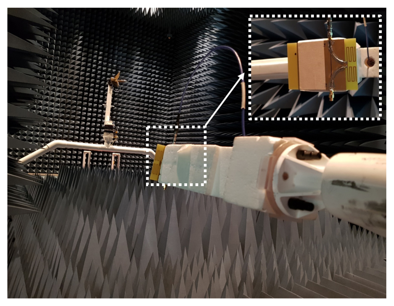
Measurement setup for the far-field radiation characteristics of the prototype antennas in an electromagnetic anechoic chamber.

Fig. 6 presents the ECC values computed using the simulated and measured 3D radiation patterns. The slight deviations between the simulation and measurement could have originated from the difference between the chamber testing environment and the ideal simulation.

Fig. 6

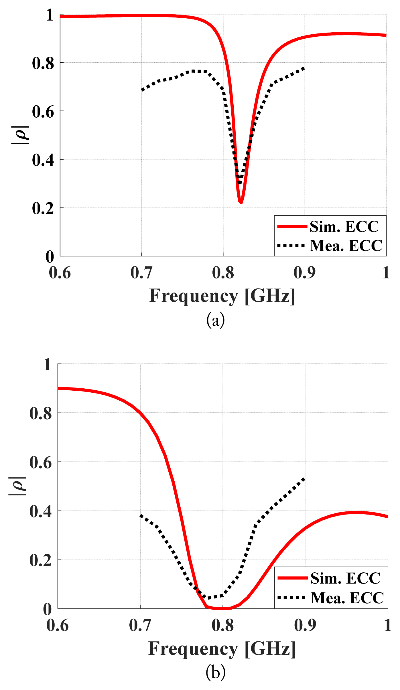
Comparison of the ECC between the simulation and measurement results of the prototype antenna: (a) high ECC model and (b) low ECC model.

For the high ECC model (Fig. 6(a)), ECC is low at 0.82 GHz but high at 0.8 GHz as intended. The measured ECC value at 0.8 GHz is 0.69 for the low ECC model (Fig. 6(b)). At 0.8 GHz, the measured ECC value at 0.8 GHz is only 0.076 and shows a broader frequency range exhibiting the null.

III. Analysis of the ECC Reduction Effect by the Suspended Line

Having verified that the full-wave simulation results and measured results showed similar tendencies, we analyzed the ECC reduction effect by calculating the surface current densities (J_surf) on the suspended line. For this purpose, the observation points for calculating J_surf on the suspended line of the high/low ECC model were set up. As shown in Fig. 7(a) and (b), the center of the suspended line was chosen for the high and low ECC models, respectively.

Fig. 7

Surface current density calculation point for the (a) high ECC model and (b) low ECC model.

Fig. 8(a) shows the calculated magnitude of J_surf at the center point 1 for the high and low ECC models. It is interesting to note the abrupt changes at the lowest ECC frequency. The null of the ECC of the two models was located at the point where the magnitude of the surface current density changed sharply. On this basis, we can confirm that the two indicators have a certain relationship. To further analyze the relationship between J_surf and ECC, the magnitude of J_surf was differentiated with respect to the frequency and then compared with the ECC curves, as presented in Fig. 8(b).

Fig. 8

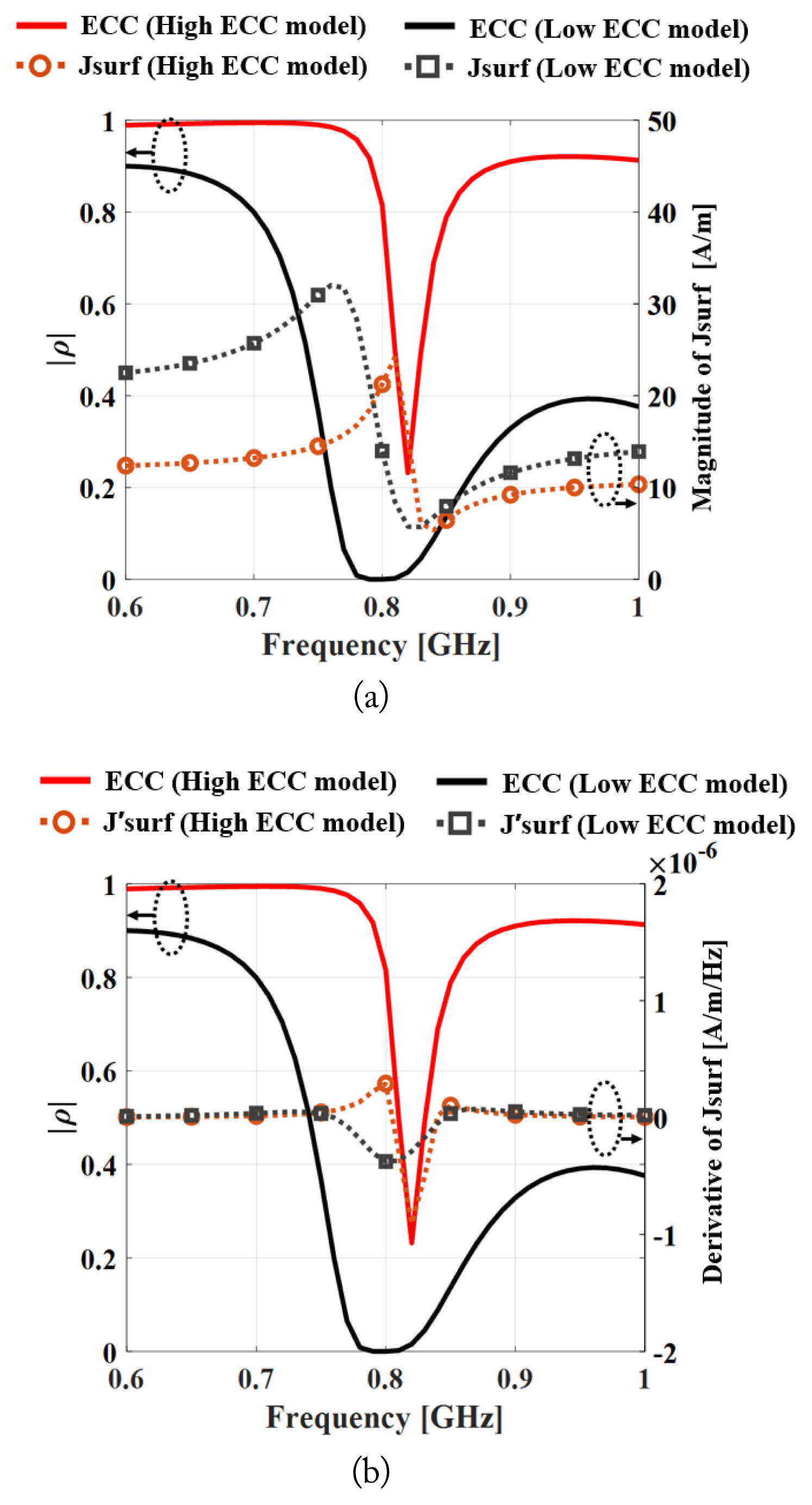
Comparison of the ECC and J_surf calculated at point 1: (a) ECC and magnitude of J_surf and (b) ECC and derivative of J_surf.

The differentiated response of J_surf showed a phenomenon in which the value rapidly decreased at the minimum ECC frequency, while a constant value was maintained. This result supports the cancellation of the surface currents flowing from one antenna to another due to a 180° out-of-phase condition as the frequency varies.

For the high ECC model, the 180° out-of-phase frequency band (i.e., J_surf abruptly changing band) is narrow and located next to the frequency of interest (0.8 GHz). Therefore, the ECC at 0.8 GHz is high. Conversely, the 180° out-of-phase band of the low ECC model is smooth and broad, resulting in a broader low ECC frequency response.

We performed a parametric study to further investigate the relationship between the ECC and the derivative of J_surf. Specifically, the length of the suspended line and the length of the antenna, which greatly affect the MIMO antenna’s ECC, were set as the design parameters, as shown in Fig. 9. Accordingly, L was set as the variable for adjusting the length of the antenna, and YY was set as the variable for adjusting the length of the suspended line. As the width of the antenna and the thickness of the suspended line had no significant effect, they were not considered as design parameters for the parametric study.

Fig. 9

Design parameters for parametric studies: (a) high ECC model and (b) low ECC model.

Fig. 10 presents the parametric study results of the high ECC model. For the parametric study, the L and YY values of the high ECC model were varied from 25.5 mm to 29.5 mm and from 5.5 mm to 9.5 mm, respectively, and the resulting variation profiles for the ECC and the derivative of J_surf were shown. Fig. 10(a), (b), and (c) illustrate the variation of the ECC and the derivative of J_surf according to the change in the design variable L. As the L value increases, the null of the two indicators shifts to the low-frequency band, similar to the decrease in antenna resonant frequency shifts as the antenna length increases.

Fig. 10

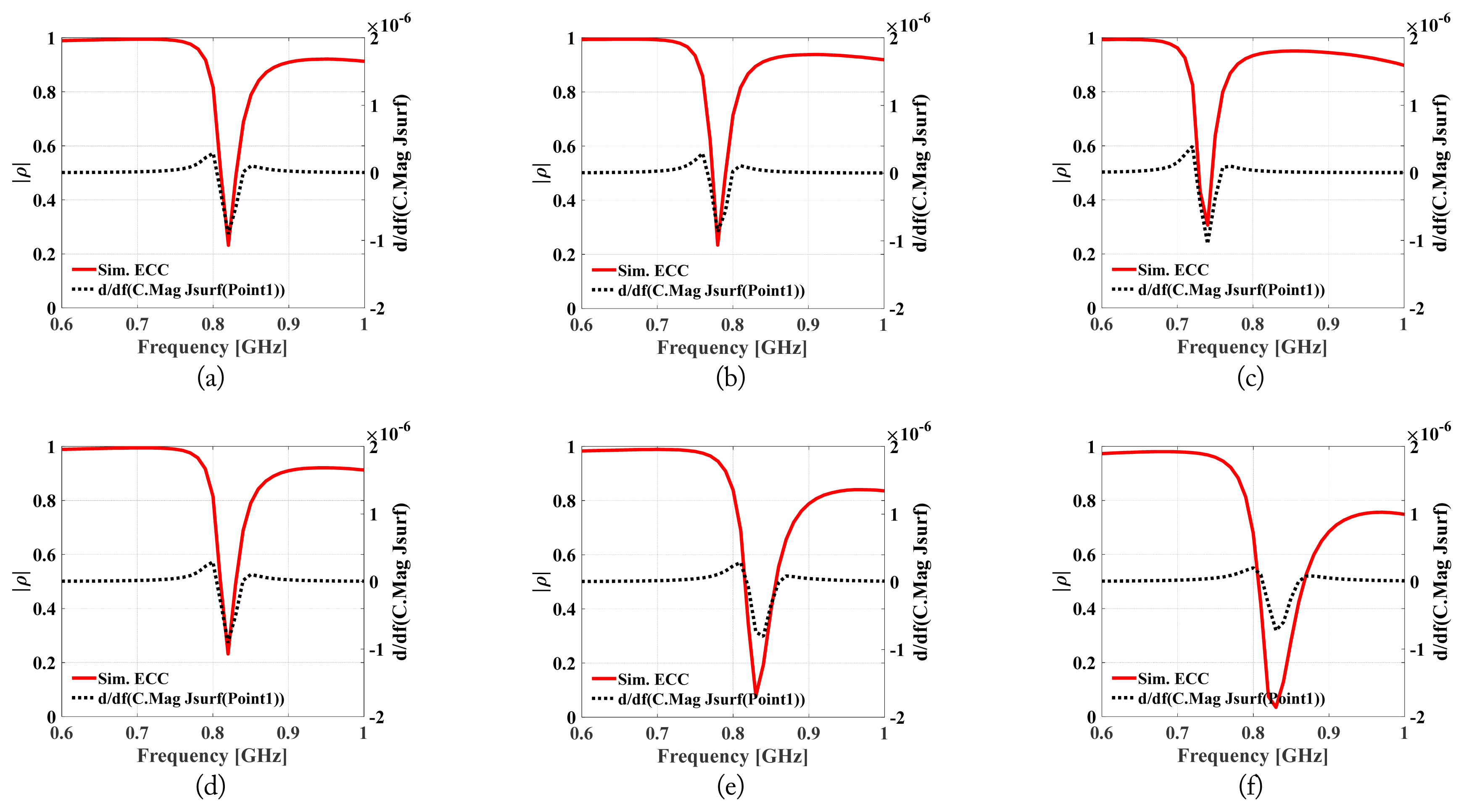
Variation of the ECC and the derivative of J_surf according to the change in design parameters of the high ECC model. (a) L = 25.5 mm, (b) L = 27.5 mm, (c) L = 29.5 mm, (d) YY = 5.5 mm, (e) YY = 7.5 mm, (f) YY = 9.5 mm.

Fig. 10(d), (e), and (f) illustrate the variation in the ECC and the derivative of J_surf according to the change in the design variable YY. As YY increases, the bandwidth around the null of the ECC widens from 50 MHz to 70 MHz. This phenomenon occurred because the impedance of the suspended line decreased as the YY value increased, and accordingly, the amount of the surface current flowing through the suspended line changed. Considering the above, the ECC minimum frequency and bandwidth can be controlled by L and YY, which are the length of the antenna and suspended line, respectively.

In the same way, we performed a parametric study on the low ECC model, and the results are presented in Fig. 11. For the parametric study of the low ECC model, the L and YY values were varied from 23.7 mm to 27.7 mm and from 12.5 mm to 16.5 mm, respectively. Fig. 11(a), (b), and (c) illustrate the variation of the ECC and the derivative of J_surf according to the change in L. Similar to the high ECC model, as the L value increases, the null of the two indicators shifts together to the low-frequency band.

Fig. 11

Variation of the ECC and the surface current, which is differentiated in terms of frequency according to the change in the design parameters of the low ECC model. (a) L = 23.7 mm, (b) L = 25.7 mm, (c) L = 27.7 mm, (d) YY = 12.5 mm, (e) YY = 14.5 mm, (f) YY = 16.5 mm.

Fig. 11(d), (e), and (f) show the variation of the ECC and the derivative of J_surf according to the change in YY. As YY increases, the bandwidth around the null of the two indicators widens from 100 MHz to 140 MHz. From the parametric study results of the two models for the design variable YY, the length of the suspended line determines the low ECC bandwidth.

IV. Conclusion

In this paper, we analyzed the relationship between ECC, J_surf, and its derivative of a MIMO antenna connected with a suspended line. A pair of two-port MIMO antenna models exhibiting high and low ECC values were designed by inserting a short and long suspended line between the antenna elements. For each model, the antenna prototype was fabricated, and its S-parameters and radiation patterns were measured. With the measured 3D radiation patterns, the ECC was calculated and compared with the simulation results. The ECC reduction effect could be clearly observed in different ways for the high and low ECC models. The high ECC model showed an abrupt change in ECC along the frequency, whereas the low ECC model showed a relatively smooth change in ECC, resulting in a wider ECC minimum bandwidth.

These abrupt and smooth variations along the frequency turned out to be related to the profile of the J_surf magnitude and its derivative in terms of frequency. This dispersive phenomenon is similar to the group delay, which is the phase derivative in terms of frequency. In fact, the ECC reduction effect due to the suspended line can be explained by the negative group delay phenomenon with a circuit, including lossy loads [13]. The latter can be considered as the MIMO antennas with high-radiation losses for the current study. By adding the suspended line, which is low loss, between these lossy antennas, the overall circuit becomes highly dispersive, and the group delay between the two ports exhibits a negative sign in a limited frequency range (i.e., the phase of S₂₁ increases as the frequency increases).

To further investigate the relationship between the ECC and the derivative of J_surf, the changes in these two indicators were observed by varying the length of the MIMO antenna and that of the suspended line. The results show that the ECC minimum frequency can be adjusted by the antenna length and that the ECC minimum frequency bandwidth is controllable by the suspended line length. We believe that these results can provide meaningful insights for MIMO antenna designers in the field.

Article information Continued

References

Biography
Seung-Ho Kim received his B.S. and M.S. degrees from the Department of Electrical and Information Engineering, Seoul National University of Science and Technology in 2017 and 2019, respectively. He currently works at Hyundai Motor Company. His research interests include antenna and RF circuit designs.
Jae-Young Chung received his B.S. degree from Yonsei University, Seoul, South Korea, in 2002, and his M.S. and Ph.D. degrees from the Ohio State University, Columbus, OH, USA, in 2007 and 2010, respectively, all in electrical engineering. From 2002 to 2004, he was an RF engineer in Motorola Korea. From 2010 to 2012, he was an antenna engineer in Samsung Electronics. He is currently an associate professor at the Department of Electrical and Information Engineering, Seoul National University of Science and Technology. His research interests include electromagnetic measurement and antenna design.