An Improved Semi-Empirical Model for Radar Backscattering from Rough Sea Surfaces at X-Band
Article information
Abstract
We propose an improved semi-empirical scattering model for X-band radar backscattering from rough sea surfaces. This new model has a wider validity range of wind speeds than does the existing semi-empirical sea spectrum (SESS) model. First, we retrieved the small-roughness parameters from the sea surfaces, which were numerically generated using the Pierson-Moskowitz spectrum and measurement datasets for various wind speeds. Then, we computed the backscattering coefficients of the small-roughness surfaces for various wind speeds using the integral equation method model. Finally, the large-roughness characteristics were taken into account by integrating the small-roughness backscattering coefficients multiplying them with the surface slope probability density function for all possible surface slopes. The new model includes a wind speed range below 3.46 m/s, which was not covered by the existing SESS model. The accuracy of the new model was verified with two measurement datasets for various wind speeds from 0.5 m/s to 14 m/s.
I. Introduction
An accurate theoretical model for radar backscattering from sea surfaces is required for various applications, such as accurate remote sensing of wind speed, wind direction, and oil spills at sea. Among many theoretical scattering models, the semi-empirical sea spectrum (SESS) model is the most widely used [1]. However, the existing SESS model has been valid only for wind speeds of U > 3.46 m/s, which led us to develop a new model that works at wind speeds of U < 3.46 m/s as well as for other ranges of wind speed.
The integral equation method (IEM) model is quite accurate for radar scattering from small-roughness surfaces [2]. To apply the IEM model for backscattering from sea surfaces, it was attempted in [3] to retrieve the input roughness parameters (root-mean-square [RMS] height and correlation length of a sea surface profile) by direct data-fitting between the IEM model and various measurement datasets for various frequencies and wind speeds. However, the retrieved parameters do not agree with the physical structures of sea surfaces, and the large-roughness effect of sea surfaces was ignored in [3].
According to the measured backscattering coefficients of sea surfaces [4, 5], the backscattering coefficients show different values at different radar modes, even at same frequency. This difference might arise from variations in radar foot prints. A high-resolution (small foot print) radar will ‘see’ only a small patch of a sea surface at a time. Fig. 1 shows a profile of a sea surface that was numerically generated using the Pierson-Moskowitz ocean spectrum [6]. A synthetic aperture radar (SAR) with 3-m resolution, for example, will measure a sea surface area of only about 3 m × 3 m at a time, and consequently, it measures the radar backscatter of an inclined small-roughness surface patch (facet) with an inclination angle, as shown in Fig. 1. The inclination angle of a facet is denoted by the normal unit vector n̂. We focused on the X-band frequency, which is used by Korea Multi-Purpose Satellite 5 (KOMPSAT-5) and KOMPSAT-6.
In this paper, we assume that a sea surface is comprised of small-roughness surface facets with slopes that have the probability density function (PDF) given in [1]. The backscattering coefficient of the small-roughness surface is computed using the IEM model, and the input parameters of the IEM (RMS height and correlation length of the small-roughness surface) are retrieved from numerically generated small-roughness sea surfaces corresponding to high-frequency portions of sea spectra for various wind speeds. This slope-variant-facet (SVF) model is semi-empirically developed based on the existing SESS model, the IEM model, and the experimental datasets in [7] and was verified using the datasets in [8].
II. Extraction of Small-Roughness Parameters
The surface height roughness parameters are the RMS height (standard deviation of the surface-height PDF), correlation length (displacement for the decrease of a normalized autocorrelation function to the e−1), and a type of surface correlation function. First, ocean spectra are generated, and then cut-off frequency points can be found for the small-roughness surfaces (i.e., high-frequency spectrum regions).
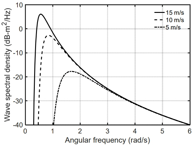
We used the Pierson-Moskowitz ocean spectrum [1, 6] in the following form: S(ω) = αg2ω−5exp[−β(ω0/ω)4], where α = 8.1 × 10⁻³, β = 0.74, g is the gravitational constant, ω0 = g/U19.5, and U19.5 is the wind speed at a height of 19.5 m. Fig. 2 shows the wave spectral densities at wind speeds of 15, 10, and 5 m/s. The peak of the spectrum is given as ωpeak = 0.877/U19.5 (e.g., ωpeak = 0.8382 rad/s at U = 10 m/s). The maximum angular frequency ωmax is set to one hundred times of ωpeak (100 ωpeak) for convenience.
We need to find a cut-off frequency ωc for generation of a small-roughness sea surface, corresponding to the range of the radian frequency of ωc ≤ ω ≤ ωmax. The cut-off frequency can be found with a trial-and-error method for each wind speed, according to the following procedure. First, we generated a small-roughness surface with a picked ωc. Second, we retrieved small-roughness parameters (RMS height and correlation length) from a numerically generated small-roughness surface. Third, we compared the backscattering coefficients of the SVF model with the data in [7]. Finally, we iterated the above procedure to get an optimum ωc for each wind speed. From this procedure, we found that the optimum cut-off radian frequency ωc is about 0.135 ωmax, or 13.5 ωpeak. For example, the optimum ωc was found to be about 11.3 rad/s at U = 10 m/s.
With the obtained optimum cut-off angular frequencies for wind speeds in a range of 0.1 m/s ≤ U ≤ 10 m/s at X-band, small-roughness sea surfaces were numerically generated. Then, we developed the following empirical expressions for the RMS height and surface correlation length as functions of wind speed, as shown in the following equations from the small-roughness sea surfaces that were generated using the Pierson-Moskowitz ocean spectrum.
where hrms is the RMS height, lc is the correlation length, U is the wind speed, and φ is the azimuthal angle (e.g., φ = 0° corresponds to the up-wind direction).
III. Development of the Scattering Model
The nth-power roughness spectrum (Fourier transform of the nth-power of correlation function) is required for the IEM model [2]. Since sea surfaces usually show an exponential-like correlation function, we utilized the modified roughness spectrum for an exponential function in the following form [3]:
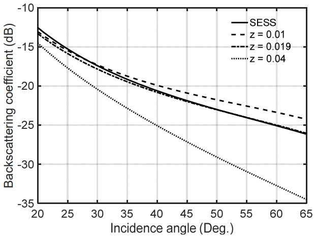
where z is a decay factor that can be chosen appropriately, L is the correlation length, K is 2ksinθ, and k is the wave number. Fig. 3 shows a comparison between the SVF model and the existing SESS model in choosing the decaying factor z. As an example, for a wind speed of 4 m/s, the optimum z value is about 0.019, as shown in Fig. 3.

Comparison between the SVF model and the SESS model for various z values with a wind speed of 4 m/s at 8.91 GHz and VV-polarization.
Based on the IEM model for small-roughness sea surfaces, we propose the SVF model in the following form, along with the slope PDF for the effect of large-roughness sea surfaces.
where σ0IEM-pp(θ′,φ) represents the backscattering coefficients computed by the IEM model [2, 3] for small-roughness facets and Pθ (Zx′,Zy′) is the slope PDF in [1]. In order to use IEM with a small-roughness condition, the khrms value must be less than 3, where k is the wave number and hrms is the RMS height. The local incidence angle θ′ can be computed using the normal unit vector of the facets:
where
and
where Zx and Zy are the surface slopes in x and y directions (i.e., Zx = ∂Z(x, y)/ ∂x and Zy = ∂Z(x, y)/ ∂y, where Z(x, y) is the sea surface height).
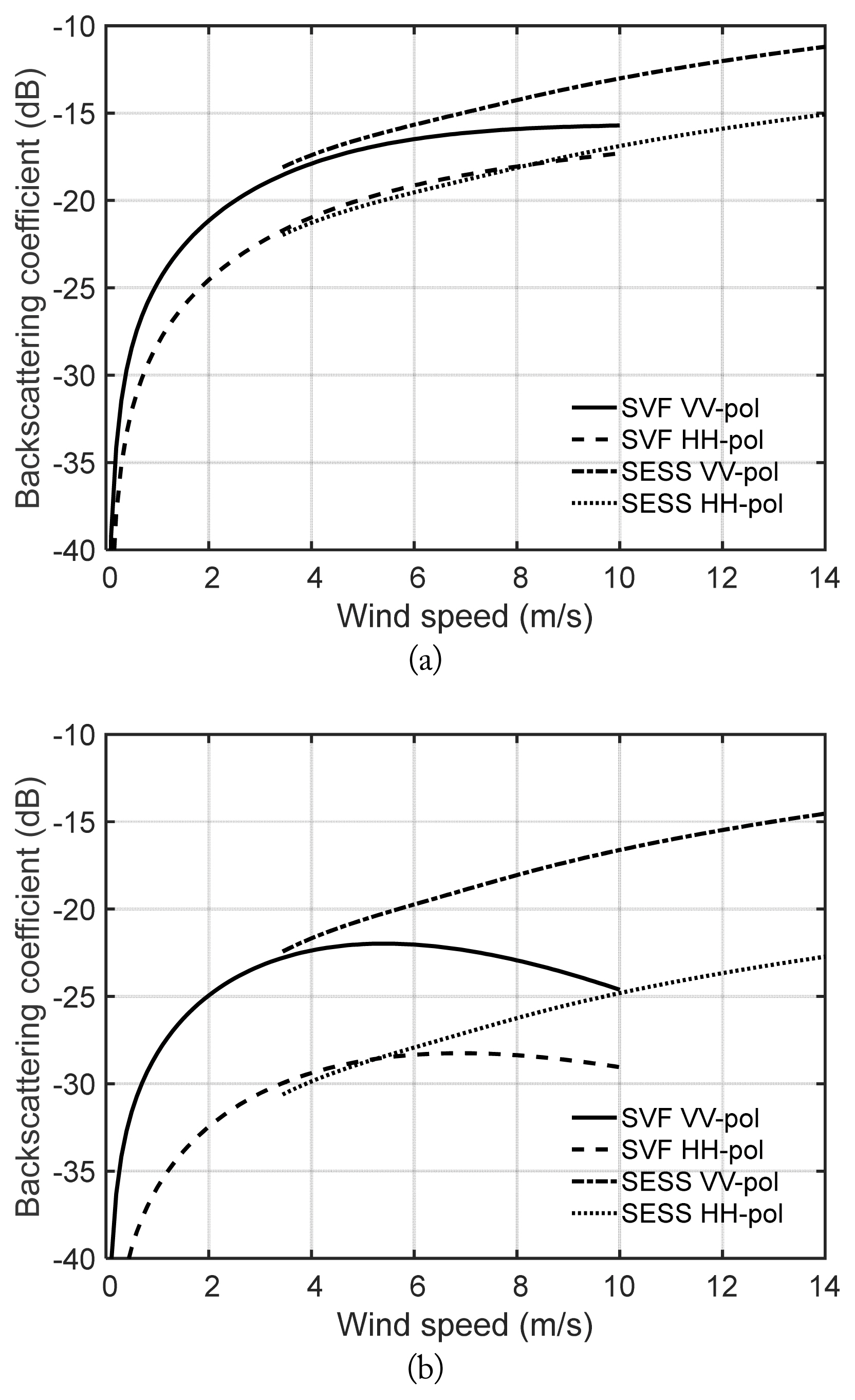
Fig. 4 shows the superposition of the SESS model [1] and the SVF model in Eq. (4) for various wind speeds at X-band frequencies at (a) θi = 30° and (b) θi = 45°. Our primary goal is to extend the validity region of the SESS model to lower wind speeds. In Fig. 4, the lines of the SVF model and the SESS model intersect at about U = 3.5 m/s for VV and HH polarizations at θi = 30° and θi = 45°, as shown in Fig. 4(a) and (b). Therefore, we propose a new semi-empirical model for X-band radar backscattering from the sea surface by combining the SVF model and the SESS model in the following form.

Superposition of the new model and the SESS model for various wind speeds at 8.91 GHz at (a) θi = 30° and (b) θi = 45°.
where σ0SVF is given in Eq. (4); σ0SESS is given in Eq. (18) in [1].
IV Verification of the New Model
The new scattering model is comprised of the new SVF model for lower wind speeds and the existing SESS model for higher wind speeds, as in Eq. (8). We examined the accuracy of the new scattering model using an experimental dataset [7], which was also used in developing the model, and an additional independent dataset in [8]. Fig. 5(a) and (b) show comparisons between the new model and two datasets in [7, 8] at θi = 0° and θi = 45°. The first dataset [7] has 26 data points for each VV-and HH-polarization, and the second dataset [8] has a total of 35 data points for various wind speeds.

Comparison between the new model and the measurements for various wind speeds at 8.91 GHz at (a) θi = 30° and (b) θi = 45°.
The datasets in Fig. 5 were acquired in an upwind direction. The model is generally in agreement with the experimental datasets, although the data points are quite scattered around the model curves, as shown in Fig. 5(a) and (b) for θi = 30° and θi = 45° at X-band. The root-mean-square errors (RMSEs) have been computed with (∑(M–d)2/N)0.5, where M is the model values, d is the data, N is the amount of data. The RMSE of the first dataset [7] at θi = 30° for VV- and HH-polarizations are 2.50 dB and 2.29 dB, those at θi = 45° for VV and HH polarizations are 5.77 dB and 3.70 dB, and the RMSEs of the second dataset [8] at θi = 30° and θi = 45° for VV- polarization are 2.93 dB and 4.53 dB, respectively.
The new model might be well applicable for radar backscattering from sea surfaces for X-band radar systems at various wind speeds. It should be noted that for a given radar system with a specific resolution (or foot print) according to an antenna beam-width, radar height, and incidence angle, the small-roughness parameters must be retrieved only once based on the first measurement dataset to increase the accuracy of the new model, especially at frequencies other than X-band. It should be also noted that the decaying factor z in Eq. (3) can be extracted only once by comparing the model with the first measurement dataset to increase the accuracy of the model.
V. Conclusion
A new semi-empirical model for radar backscattering from sea surfaces is proposed in this paper. The SVF model was developed for lower wind speeds using the following approach: we (1) extracted the small-roughness parameters from numerically generated sea surfaces for various wind speeds, (2) used the IEM model to compute the small-roughness-scale backscattering coefficients for various wind speeds, (3) calculated the backscattering coefficients by integrating the IEM results multiplied with the surface slope PDF to account for the large-roughness characteristics, and (4) iterated the above procedure to get the optimum small-roughness parameters (RMS height and correlation length) for each wind speed. The final form of the semi-empirical model was obtained by combining the new SVF model and the SESS model to extend the validity region of the latter. Another advantage of the new model is its ability to adapt radar specifications, such as the radar resolution or foot print, to increase the accuracy of the semi-empirical model. It was shown that the new model agrees quite well with the experimental data at X-band for VV- and HH-polarizations.
Acknowledgments
This research was supported by the Basic Science Research Program of the National Research Foundation of Korea (NRF) (No. 2016R1D1A1A09918412).
References
Biography
Taekyeong Jin received a B.S. degree in electronic and electrical engineering from Hongik University, Seoul, Korea, in 2017. He is currently working toward an M.S. degree in the Department of Electronic and Electrical Engineering, Hongik University, Korea. His research interests include microwave remote sensing and array antennas.

Yisok Oh received a B.S. degree from Yonsei University, Seoul, Korea, in 1982, an M.S. degree from the University of Missouri, Rolla, MO, USA, in 1988, and a Ph.D. degree from the University of Michigan, Ann Arbor, MI, USA, in 1993, all in electrical engineering. In 1994, he joined the faculty of Hongik University, Seoul, where he is currently a professor in the School of Electronic and Electrical Engineering. His current research interests include polarimetric radar backscattering from various Earth surfaces and microwave remote sensing of soil moisture and surface roughness.


