


I. INTRODUCTION
Investigations into scattered waves arising from different objects and cavities offer useful insights for the design of electromagnetic structures used in practical applications, including optics, non-destruction testing, remote sensing, and radar cross section (RCS) reduction. Multiple methods have been proposed for analyzing the scattering of electromagnetic (EM) waves induced by various types of opened cavities, such as rectangular grooves [1ŌĆō5], circular-arc channels [6ŌĆō8], and triangular grooves [9ŌĆō11].
EM scattering by elliptical cavities have also been conducted [12ŌĆō14]. A simple closed-form solution for the scattering generated from a semi-elliptic groove in the low-frequency limit was derived in [12], which was found to be valid for arbitrary polarization, arbitrary incidence and scattering directions, as well as arbitrary eccentricity. In [13], an analytic series solution based on the mode-matching technique was proposed for a semi-elliptic groove. Furthermore, [14] derived an analytic solution to the problem of scattering using a dielectric-coated conducting elliptic cylinder loading an elliptic groove in a perfect electric conductor (PEC). However, these solutions are only usable in the case of simple elliptic cavities. To calculate electromagnetic waves in a complex structure, such as elliptical boundaries, it seems reasonable to employ full numerical methods, such as the finite element method and the method of moment (MoM) meshing technique. However, when the size of the structure increases, the refinement of its grids produces enormous systems, solving which is computationally expensive.
This paper develops an efficient semi-analytic method to solve the issue of EM scattering originating from a truncated semi-elliptic cavity embedded in a PEC ground plane. The solution is based on boundary value analysis [13] and the region-point-matching method [15], which is a numerical matching procedure. As a result, the proposed method simultaneously benefits from the advantages of both the numerical and analytical methods. Furthermore, this methodology is easily applicable to complex problems related to elliptic boundaries, for which the Mathieu function addition theorem, characterized by difficult series and equations, has mostly been used. The Mathieu functions represent the solution to the wave equation with elliptical boundary conditions [16]. In 1868, Emile Mathieu presented a new differential equation, called the Mathieu equation, whose eigenvalues and corresponding periodic solutions led to the definition of a new class of functions, known as the Mathieu functions. Later, Whittaker and others developed novel theories and methods to compute the Mathieu functions [16ŌĆō19].
The steps involved in addressing the problem being dealt with in this research are as follows: first, two semi-elliptical auxiliary boundaries are introduced, following which the analyzed region is divided into three sub-regions. The tangential fields in the three sub-regions are expanded according to the Mathieu functions. By imposing matching boundary conditions at the first auxiliary interface (between sub-regions 1 and 2) and applying the orthogonal properties of the angular Mathieu functions, two sets of linear equations are analytically obtained. In the next step, the boundary conditions at the second semi-elliptical auxiliary border (between sub-regions 2 and 3) are satisfied by uniformly collocating the points in two different coordinate systems, leading to the construction of two other sets of linear equations. In this context, it is noteworthy that the collocation method is used to match the tangential fields for the purpose of avoiding the complex application of the addition theorem. Finally, the solution is summarized as a set of infinite algebraic equations that can be solved numerically by truncating infinite equations. Following this, the proposed method is compared to the MoM method used in the FEKO software to validate the obtained results. Finally, the effects of the cavity depth and incidence angle on the EM scattering signature are investigated.
II. THEORETICAL FORMULATION
1. Description of Cavity
This study considers a semi-elliptical open cavity embedded in a PEC that is horizontally truncated at the bottom, as shown in Fig. 1. Two Cartesian coordinate systems and its two corresponding elliptic cylinder coordinate systems are also presented in Fig. 1. The origin of the global coordinate systems (x, y) or (╬Š, ╬Ę) is fixed at the center of the elliptic cavity, while the origin of the local coordinate system (x1, y2) or (╬Š1, ╬Ę1) is placed at the midpoint of the cavity bottom. The half lengths of the major and minor axes and the focal distance of the elliptic cavity are a, b, and c, respectively. Furthermore, the truncation depth of the semi-elliptical cavity is denoted as d, while the bottom width is referred to as 2W. The two lower corners of the cavity are located at ╬Ę = ŌłÆ╬Ęb and ╬Ę = ŽĆ + ╬Ęb with respect to the global elliptic coordinate. In the case of the two semi-elliptical auxiliary borders, the semi-elliptical boundary S1 is defined as {(╬Š, ╬Ę)|╬Š = ╬Šc0}, based on which the second half of the curve forms the cavity wall, and the semi-elliptical boundary S2 is considered {(╬Š1, ╬Ę1)|╬Š1 = ╬Šc1}, where the half lengths of the major and minor axes and focal distance of S2 are W, b1, and c1, respectively. As shown in Fig. 1, by introducing the auxiliary boundaries S1 and S2, the analyzed region can be divided into three sub-regionsŌĆöan open region (Region 1) and two enclosed regions (Regions 2 and 3). In this context, it should be noted that the interface S2 should satisfy two important conditions:
1) It should not cross the interface S1.
2) The origin of o should be placed below the border S2 inside Region 2.
To satisfy these conditions, d < b1 Ōēż b ŌłÆ d is considered. Notably, the shape of the boundary S2 can be altered as desired by changing its axial ratio.
2. Electric Field Expansion in Region 1
A transverse-magnetic (TM) polarized plane wave can be expressed as follows:
where the suppressed time dependence of exp (jŽēt) is incident on a truncated semi-elliptic cavity with the incidence angle ŽĢi, as shown in Fig. 1, where k0 is the free-space wave number. In the open Region 1, the sum of the incident and reflected fields in the global coordinate system (╬Š, ╬Ę) can be expanded using the Mathieu functions as follows:
where q is (k0a e)2/4. Furthermore,
M s n ( 1 ) ( . )
Subsequently, the total electric field
E z I ( ╬Š , ╬Ę )
(4)
where An refers to the unknown coefficients that need to be determined.
3. Electric Field Expansion in Region 2
As mentioned previously, the center of the semi-elliptical boundary S1 is located outside Region 2. Therefore, there are no singular points in this region, which indicates that the z-components of the electric field in this region can be expressed using a proper wave function, as follows:
(5)
where
M c n ( 1 ) ( . ) , M c n ( 4 ) ( . )
4. Electric Field Expansion in Region 3
Region 3 comprises a semi-elliptical auxiliary boundary S2 and a flat PEC boundary at the bottom of the cavity (╬ōb). According to the coordinate system (╬Š1, ╬Ę1), the electric field
E z ( I I I ) ( ╬Š 1 , ╬Ę 1 )
where q1 is (k0W e1)2/4. Notably, the complex expansion coefficients Fn are unknown.
5. Boundary Conditions Applying
Before applying the boundary conditions, it is necessary to obtain the tangential component of the magnetic field. The tangential magnetic field H╬Ę in each region is derived using MaxwellŌĆÖs equations, as follows:
The tangential fields in Regions 1, 2, and 3 should satisfy the following boundary conditions:
(8)
(9)
By applying the six boundary conditions, the unknown coefficients An, Bn, Cn, Dn, En and Fn can be obtained. The above expressions show that Eqs. (8), (10), and (11) are expressed in the elliptical coordinate system (╬Š, ╬Ę), while the equations pertaining to (9) are in two different elliptical coordinate systems. In such a case, the Mathieu function addition theorem is the first solution that is usually considered for transferring the Mathieu functions located in multiple elliptical coordinate systems. However, this theorem is extremely challenging to employ. This study proposes a solution to avoid this difficulty by using the region-point matching technique at border S2.
6. Equations Solving
To solve Eqs. (8)ŌĆō(11) for the unknown expansion coefficients, both sides of Eqs. (8), (10), and (11) are first multiplied by sem(╬Ę, q) and then integrated with the corresponding boundary to obtain four independent linear equations, as follows:
(12)
(13)
(14)
(15)
where ╬┤nm is the Kronecker delta, while functions Znm, Ynm, Knm, Lnm, and Inm have been defined in Appendix. Furthermore, the prime (ŌĆ▓) notation is used to signify differentiation with respect to the corresponding function. Subsequently, to convert Eq. (9) into linear equations, point collocationŌĆöa mesh-free technique where the electric and magnetic fields are matched at discrete places at S2, whose residuals are zeroŌĆöis used. For this purpose, a sequence of points along S2 is uniformly considered. The coordinate of the mth collocation point on S2 in coordinate systems (╬Š1, ╬Ę1) and (╬Š, ╬Ę) are represented as (╬Šc1, ╬Ę1m) and (╬Šm, ╬Ęm), respectively. To convert the coordinate (╬Šc1, ╬Ę1m) into coordinate (╬Šm, ╬Ęm), coordinate (╬Šc1, ╬Ę1m) was first transformed from elliptic to Cartesian coordinates using the following expressions:
Assuming d is the distance between coordinate systems (x, y) and (x1m, y1m), xm = x1m and ym = y1m + d. The formulas to transform from Cartesian to elliptic coordi-nates, as noted in [25], are as follows:
Notably, parameters pm and rm in (17) can be defined as follows:
where
B m = x m 2 + y m 2 - c 2
(19)
(20)
To compute the unknown coefficients numerically, it is essential to truncate the infinite series in (12)ŌĆō(15) into finite numbers. Therefore, in Eqs. (12)ŌĆō(15), the summation index n is truncated into M terms. The truncated term number M depends on the accuracy requirement. Subsequently, Eqs. (12)ŌĆō(15) and (19)ŌĆō(20) constructed a set of linear systems with regard to the unknown expansion coefficients (An, Bn, Cn, Dn, En and Fn) and could be solved by matrix methods. Finally, the scattered wave in Region 3 was directly calculated using (3). Meanwhile, in the far zone (╬Š ŌåÆ Ōł×),
E z s
where
Žü Ōēģ c s i n h ╬Š ŌåÆ Ōł× ( ╬Š ) Žā T M 2 D
III. RESULTS
This section presents some examples to prove the validity of the solution developed in this study for computing near and far fields. Furthermore, to examine the influence of the problem parameters, such as the incidence of the angle (ŽĢi), the observation angle (ŽĢd) and the cavity depth (d), on the scattered field, sample numerical results are presented in Figs. 2ŌĆō7.
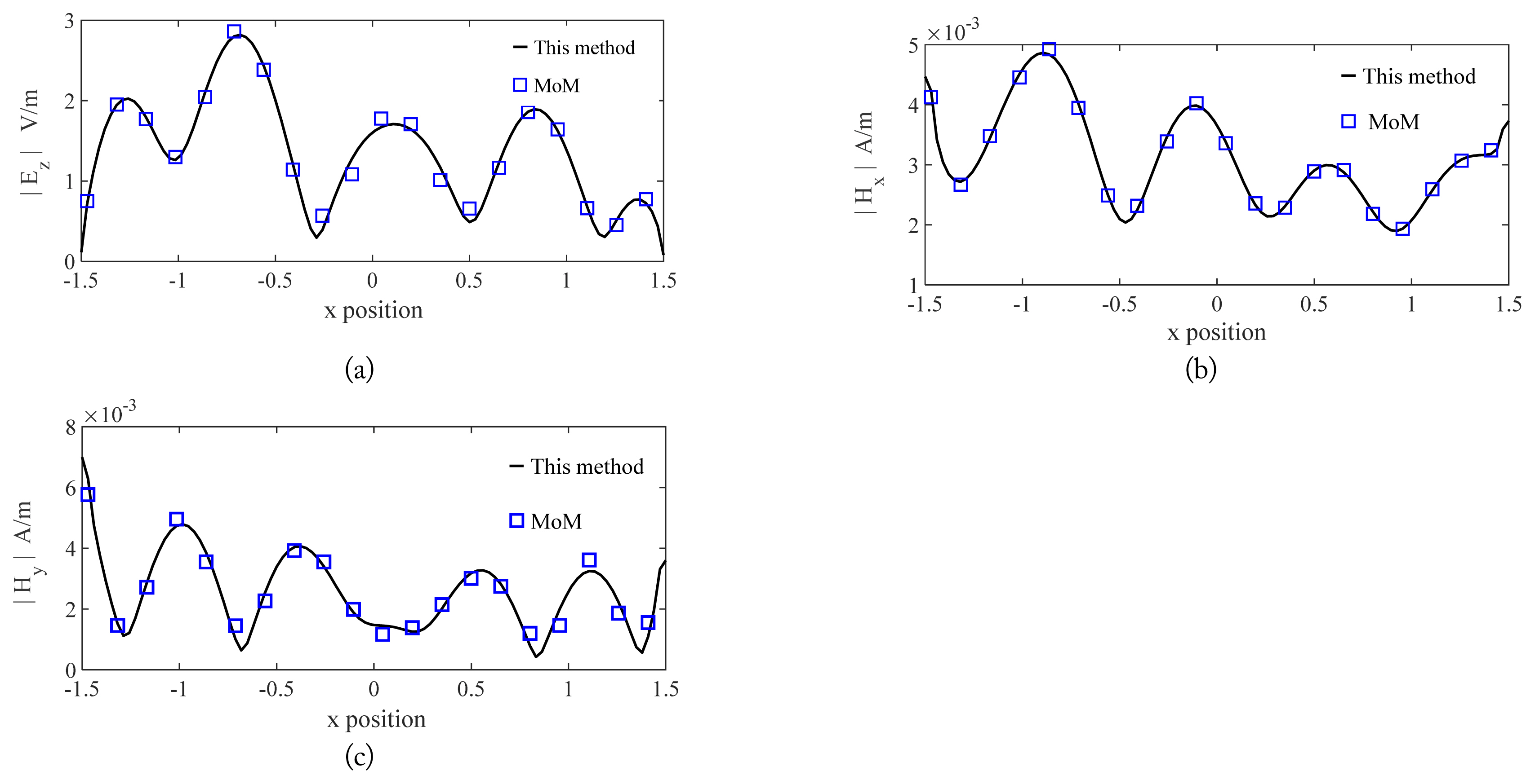
The results obtained using the proposed method were examined by comparing them to the data obtained from the FEKO software, which uses MoM. During the calculation, the infinite series had to be truncated appropriately. However, the size of the cavity is a primary factor that affects the truncation term number M. Taking this into account, this study investigated the validity of the suggested method. Fig. 2 illustrates variations in the amplitudes of the electromagnetic fields |Ez|,|Hx|, and |Hy| in terms of x position at y = 0 for the cavity presented in Fig. 1, with a/╬╗ = 1.5, b/╬╗ = 1, d/╬╗ = 0.75 when ŽĢi = 90┬░. Following this, the results shown in Fig. 3 were considered for an oblique incident case, i.e., ŽĢi = 60┬░. As shown in Fig. 2, the distribution of fields on the cavity is symmetrical for the perpendicular incident case. The results depicted in Fig. 2 were obtained using the proposed method and MoM. A comparison of the results observed in these figures demonstrates the accuracy of the proposed method. Furthermore, consequent examinations indicate that M = 50 is adequate for the given example to yield reliable results.
In the previous example, the convergence behavior of the echowidth obtained by the proposed method was verified by calculating the normalized errors of the series coefficient Am in (21) for different values of M using the following equation [22]:
The results of this exercise are plotted against the number of samples of M in Fig. 2(d), depicting that when M increases, the error increases initially and then undergoes a decline.
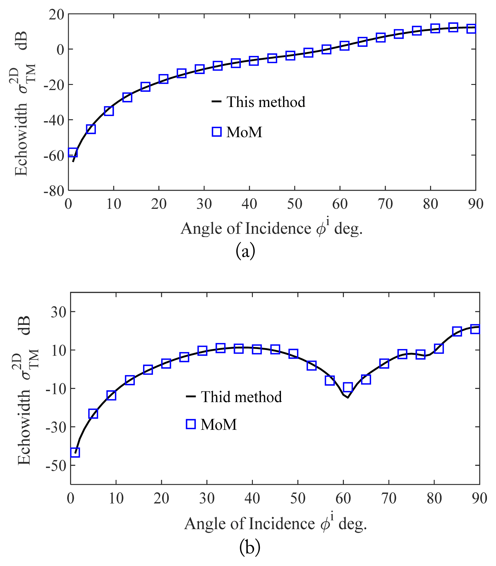
Furthermore, to study the influence of incident angle on the backscattering echowidth
Žā T M 2 D
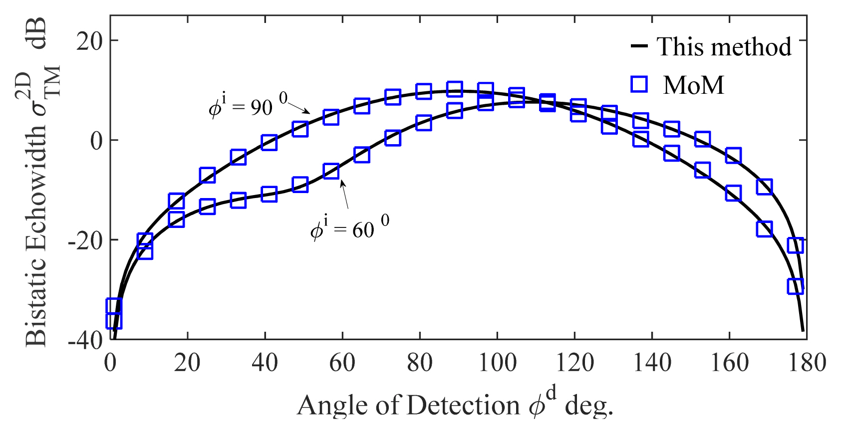
In the second case (large cavity), as shown in Fig. 4(b), a/╬╗ = 1.5, b/╬╗ = 1, and d/╬╗ = 0.75 were considered. Their echowidths were obtained, with the incident angle ŽĢi varying from 0┬░ to 90┬░. The results presented in Fig. 4 demonstrate that the scattering echowidth generally increases with an increase in the incident angle. However, in the case of the large cavity, two local minimums are observed at around ŽĢi = 60┬░ and 80┬░, where most of the energy is scattered in a direction that is different from that of the incident. Considering MoM as the reference, the results shown in Fig. 4 indicate that the proposed method is applicable to cases pertaining to both small and large cavities. Furthermore, Fig. 5 displays the TM bistatic
Žā T M 2 D
The simulation time of the proposed method and MoM (for a truncated semi-elliptic cavity with specifications as shown in Fig. 2) were calculated to conduct a comparison of the time consumed. The computing time for the proposed procedure was 7.23 seconds, while the time consumed for MoM was about 18 minutes. This indicates that the solution devised in this study enables rapid computation while also ensuring accuracy for electrically large cavities. However, computational efficiency becomes a significant problem when scattering evaluation is required for frequent simulations, such as inverse problems where a large amount of data is required to estimate the shape of a cavity or an object from scattering patterns.
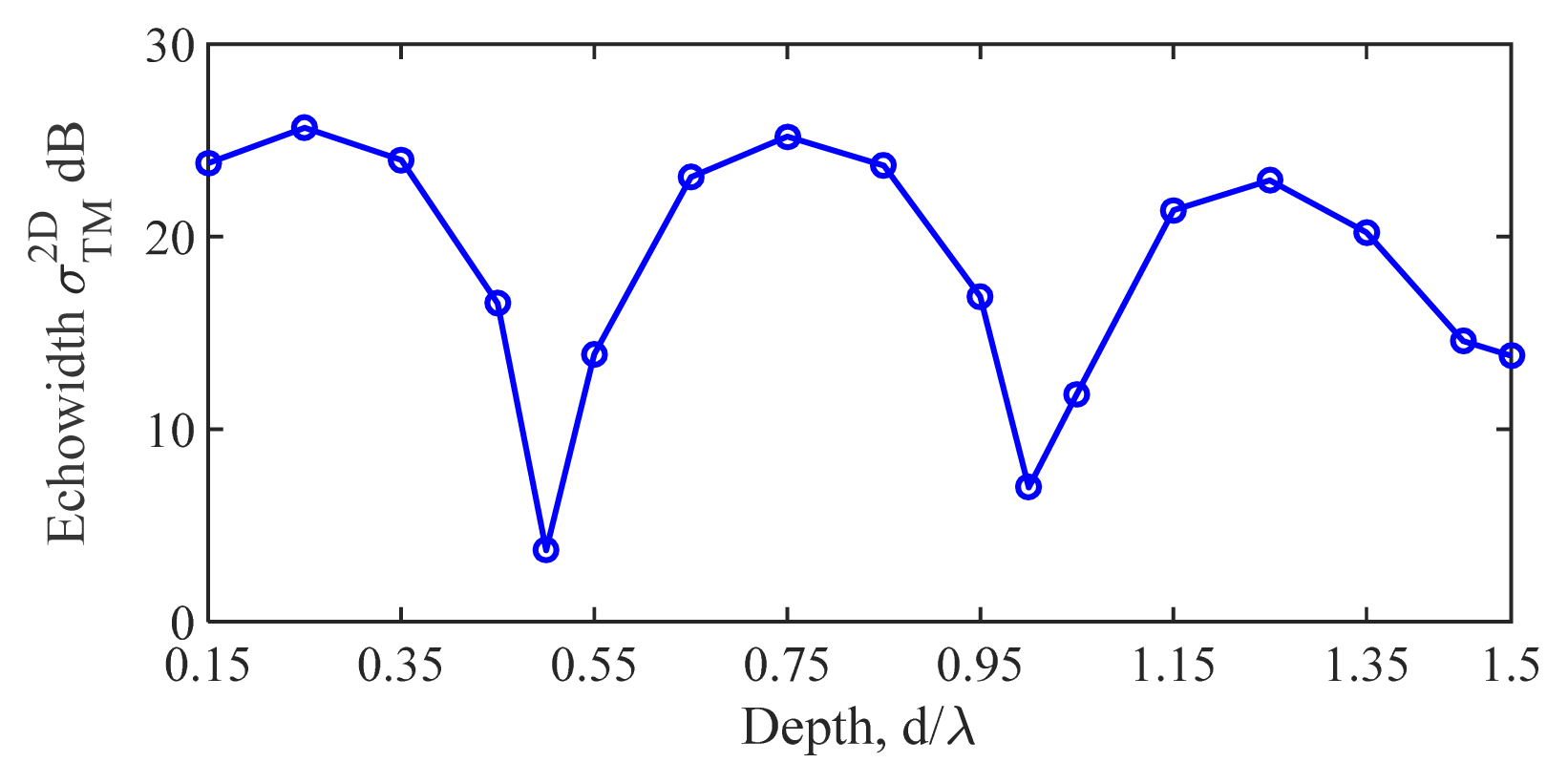
In another example, the effect of cavity depth on echowidth at normal incidence was investigated. The results of this examination are presented in Fig. 6. The specifications of the truncated semi-elliptic cavity in this example were a/╬╗ = 2, b/╬╗ = 1.5. Furthermore, the cavity depth was intially kept at d = 0.15╬╗, which was then increased by steps of 0.05╬╗ until = 1.5╬╗ was reached. Fig. 6 depicts three dips at a = 0.5╬╗, 1╬╗, and 1.5╬╗, indicating that less energy is scattered in the direction of the incidence and more is scattered in other directions in these depths.
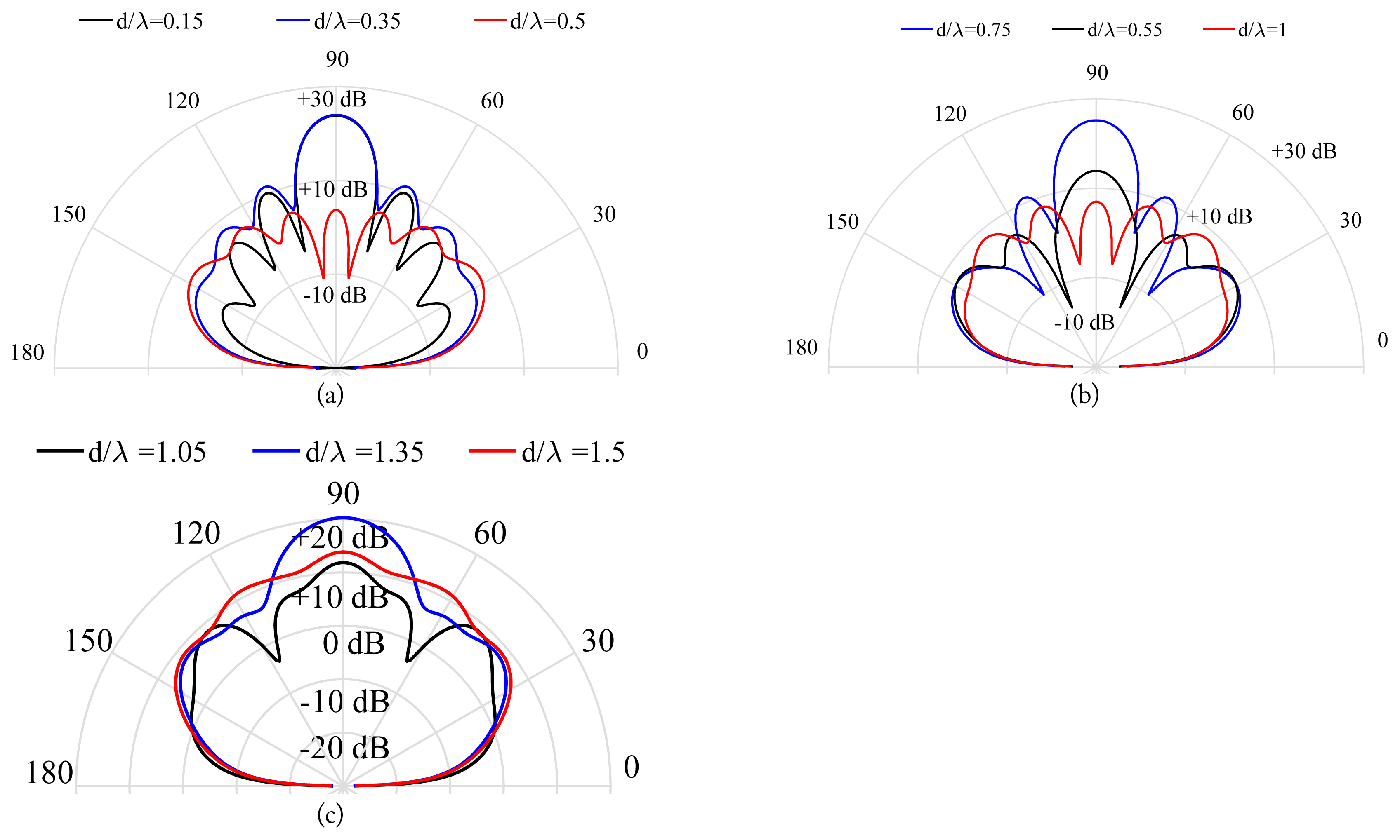
In addition, this study examined the influence of cavity depth d on the bistatic echowidth pattern. In the previous example, the bistatic echowidth of the cavity (
Žā T M 2 D
As observed in Fig. 7, the effect of the depth of the truncated semi-elliptic cavity on the scattering pattern is significant. In practice, the depth of the truncated cavity can also be considered an important parameter for controlling and shaping scattering patterns. Moreover, the results obtained in this study can be employed to design appropriate electromagnetic structures for various applications.
IV. CONCLUSION
This study semi-analytically examined the scattering waves generated by a truncated semi-elliptic cavity in a PEC using decomposition and region-point matching techniques. The described method follows a simple procedure that can be applied to address problems pertaining to elliptic boundaries, for which the Mathieu function addition theorem, which is characterized by difficult formulations, has been conventionally used. The results obtained on implementing the proposed process were compared to those obtained for the MoM used in the FEKO software. The comparison revealed that the proposed procedure is efficient and in good agreement with the results of the time-consuming and entirely numerical MoM. This study also examined the effects of cavity depth and incident angle on scattering patterns by calculating numerical results for a few typical cases.