Characterization of Induced Polarization Parameters from Electromagnetic Data using Evolutionary Approach

Article information

Abstract

I. Introduction

Interest among researchers in gaining information from interactions of electromagnetic waves with a scatterer has recently increased due to its importance in numerous science and engineering applications [1–3]. When an electrically polarizable medium is present within the scatterer, the electromagnetic (EM) response is affected by what is called “induced polarization” (IP) [4]. Induced polarization is a dynamic electromagnetic phenomenon that is directly sensitive to the electrical properties of the scatterer [5]. Extracting the induced polarization parameters from electromagnetic data provides additional information about the scatterer’s conductivity [6]. Consequently, this facilitates solutions to substantially more problems that have many applications in science and technology-related fields [7–9]. In this work, an inversion methodology is proposed to retrieve induced polarization parameters from a scattered electromagnetic field. A major challenge in inverting EM data for IP parameters is the requirement of an accurate forward model [10]. Therefore, one of the objectives of this paper is to propose a forward modeling algorithm to compute the scattered EM field in a manner that accounts for the induced polarization effect.

The other objective of this work is to propose a procedure to solve the inverse problem without affecting its nonlinear nature. This is accomplished through handling the inverse problem via an optimization procedure in which the proposed forward model can be used iteratively for different values of the unknown induced polarization parameters. Formulated as an optimization problem, the inverse problem can be tackled with one of the evolutionary approaches. Evolutionary approaches are global optimization algorithms that possess direct exploration capabilities of the entire parameters’ space. Consequently, they offer the advantages of enhancing results for highly nonlinear problems [11]. Different types of evolutionary approaches have been successively developed. Among them, the most popular are genetic algorithms (GA) [12] and simulated annealing (SA) techniques [13].

Simulated annealing is a global search approach that is able to approximate a global optimum of a given function using a limited number of control parameters. It is potentially used for approaches wherein the objective is to find an acceptable global optimum solution in a relatively large and multidimensional search space rather than to reach the exact global optimum solution [14]. Furthermore, due to its stochastic searching mechanism, it is less likely to be trapped in local minima [15]. In this work, the simulated annealing technique has been applied to solve the investigated inverse scattering problem. Different simulated annealing algorithms were designed within the proposed inversion methodology. To validate the efficiency of the inversion methodology, various different settings were considered, and the results were evaluated in terms of parameters’ estimation errors.

II. Forward Problem Formulation

In electromagnetic modeling (i.e. forward problem), one considers the problem of computing the electromagnetic data, given the physical properties of the scatterer [16]. In this paper, the forward problem is an integral part of the inversion methodology. Therefore, the efficient formulation of the forward problem is crucial for the accuracy of the inversion’s results. Here, we introduce semi-analytical forward calculations to compute the scattered electromagnetic field from the scatterer in the presence of the induced polarization effect. First, we assume a transmitter of an infinite unphased electric line source in the y direction to produce an electric field in the same direction. In this paper, we will consider a 2D scatterer model, as presented in Fig. 1, wherein the polarizable scatterer consists of an object (Ob) embedded inside a layered medium (LM). For this 2D problem, the presence of the scatterer can be represented as electric polarization and magnetic polarization currents [17]:

Fig. 1

The general model of a polarizable scatterer with an overall thickness of L.

Here, we will limit the current analysis to a case wherein the permeability μ of the scatterer is the free space permeability μ₀. Hence, for such a y-independent problem, the electric field inside the scatterer is calculated as follows [17]:

where E_ys(x, z) is the total field inside the scatterer, and Ey0(x,z) is the incident electric field. H0(1) (.) is the Hankel function of the first kind and zeroth order, k0=ωμ0 ɛ0 is the free space wavenumber, and r and r_s are the observation and source points’ locations respectively. (x, z), and (x′, z′) are observation points and electric polarization current Cartesian coordinates, respectively. Here, the double integral is on the geometry of the scatterer with L referring to the layered medium thickness along the z-direction. We can now solve the integral equation for the electric polarization current as follows:

where Q(x, z) can be written as follows:

Using the eigen solution in [18] yields Eq. (7) in the following form:

where a_n stands for the current expansion coefficient and ψ_n stands for the eigenfunction. The approach used here to solve this forward problem involves calculating the inverse Fourier transform for both sides and then multiplying by the complete set { ψm(kx′,z)} [19]. Subsequently, by making use of the orthogonality of the complete discrete orthonormal set {ψ_n (k_x, z)}, and its properties [20], we can calculate the current expansion coefficients in the following form:

where

Furthermore, for the investigated scatterer, we can define Q(x, z) as Q(x, z) = Q₁ + Q₂, where

everywhere in the layered medium except for the object and

everywhere inside the object:

In the presence of a polarizable scatterer, induced polarization effects can be described in terms of frequency-dependent complex conductivity, where the frequency dependence can be calculated using the most commonly used Cole–Cole model as follows [21]:

where η is a physical parameter called “chargeability,” which quantifies the intensity of the induced polarization effects within the medium. τ is the characteristic time constant, and c is the Cole–Cole exponent term, which refers to the degree of frequency dependence. σ_∞is the conductivity at infinite frequency or in the absence of IP effects [22].

By approximating ∫-∞∞dkx≈Σs δkx with S terms in equation (10), and by truncating Σ_n with N terms, we can reformulate the scatterer polarization current expansion coefficients in the form of a linear system:

where a(k_x) is the NS length vector, and u(k_x) is the NS length vector. D(k_x) is a square matrix of dimensions NS x NS. I is a unit matrix of size NS. Here, N stands for the total number of eigenfunctions to be involved in the representation, while S represents the horizontal wavenumbers. Once the coefficients {a_n (k_x)} are computed, the scattered electric field’s distribution attained at the receiver can be written as follows:

III. Inversion Approach

The purpose of the inversion problem is to retrieve accurate values for the Cole–Cole parameters that describe the IP phenomenon, from the scattered EM field. As the EM response is a nonlinear function of the Cole–Cole model parameters [23], an estimation of these parameters should be performed using a nonlinear inverse approach. This is accomplished by rearranging the nonlinear inversion problem into a global optimization process, wherein optimization is conducted by minimizing the objective function, ζ, defined as follows:

where Emw is the electric field obtained at the w^th wavenumber, and W represents the total wavenumbers to be included. Ecw is the electric field calculated for the w^th wavenumber based on an estimation of the 4O induced polarization properties of the scatterer. Therefore, the objective function is the 4O dimensional function in the following form:

where η_o, σ_∞o, τ_o, and c_o are the chargeability, the conductivity at an infinite frequency, the time constant, and the Cole–Cole exponent of the o^th object respectively. Here, the developed forward approach is used as an integral part of the inversion approach to iteratively minimize the multidimensional objective function through a simulated annealing approach. The simulated annealing algorithm starts with a random initial solution derived from the 4O Cole–Cole parameter’s estimates, which are the current estimates. The algorithm then starts to explore the search space to propose new estimates from the neighborhood to generate a proposed solution, wherein the distance between the proposed estimates and the current estimates in the search space are selected based on a probability distribution that depends upon a control variable called temperature [24]. The algorithm then begins to evaluate both the current and the proposed estimates using the objective function, ζ, to determine whether the proposed solution is better or worse than the current solution.

If the proposed estimates yield a solution with an objective function value lower than the objective function value of the solution obtained by the current estimates, the proposed estimates then replace the current estimates in the new iteration. On the other hand, the algorithm may opt to accept the proposed estimates as the new current estimates, even if the proposed estimates lead to an objective function value higher than the objective function value obtained from the current estimates. By allowing these types of choices that reflect an increase in the objective function, the opportunity to explore more areas in the search space can be increased, while the probability of solution being trapped in a false local minimum can be decreased. However, these choices are made according to a specific probability, which is based on an acceptance function:

The temperature T is essential to regulate the acceptance probability of a new solution. During the simulated annealing process, to determine the optimal parameters’ estimates, T is decreased systematically according to a designed cooling schedule Tc. The cooling schedule is applied to reduce the probability of accepting inferior estimates gradually throughout the algorithm iterations to determine the ideal estimate [25]. This results in a less favorable value of the objective function and hence to an optimal or a suboptimal solution to the inverse problem. In this paper, three cooling schedules are designed and applied: a fast, Boltzmann, and exponential cooling schedule. The fast cooling schedule is defined as follows:

The Boltzmann cooling schedule is defined as follows:

Lastly, the exponential cooling schedule is defined as follows:

where T₀ is the initial temperature, γ is the cooling rate, and r = 1, 2, 3 . . . is the number of iterations.

IV. Simulation And Results

Here, the problem formulation is limited to estimate the Cole–Cole parameters for each of the objects and the layered medium, given the scattered electromagnetic fields. The scattered electromagnetic fields are collected at 11 wavenumbers. The forward model is depicted in Fig. 2, where the thickness of the layered medium is 150 m, while the thickness of the embedded object is 50 m. The electromagnetic source is located at xs=zs=0.

Fig. 2

The scatterer model in this paper.

Using the simulated annealing technique in the inversion scheme permits the direct inclusion of a priori information about the possible range for each of the Cole–Cole parameters. Generally, the chargeability η can take values between 0 and 1, while the time constant value τ is within the following range: 10⁻⁶ s ≤ τ ≤ 1 s [26]. The Cole–Cole exponent c can have values from 0.1 to c = 1, while the conductivity at infinite frequency σ_∞ is within the range from 10⁻⁴ S/m to 1 S/m [27]. In this paper, we selected 10 polarizable scatterers’ configurations that are constructed from the possible ranges of the Cole–Cole parameters. The investigated configurations are summarized in Table 1.

Table 1

Induced polarization properties of the 10 investigated configurations in this paper

To study the results of the simulated annealing approach, an error term is defined as follows:

where P_a, and P_e are the actual and the estimated values of the parameter, respectively. Furthermore, to compare the three cooling schedules’ performances, an error margin is computed 100 times for each estimated Cole–Cole parameter per cooling schedule and defined as follows:

The three designed cooling schedules use 100°C as the initial temperature and 0.95 as a cooling rate. Furthermore, in this paper, the simulated annealing algorithm is designed to seek an optimum error of 0% between the estimated, and the actual Cole–Cole parameter value. If the algorithm couldn’t achieve this optimum error value, still a stopping mechanism is imposed, where after 10, 000 iterations, the algorithm stops, and outputs the estimated Cole–Cole parameters that yields the nearest error value to the optimum.

Figs. 3 and 4 summarize the comparison between the three cooling schedules’ results and the investigated configurations in terms of the error margin of each of the Cole–Cole estimated parameters for the layered medium and the object, respectively. The comparisons in Figs. 3 and 4 reveal that, among the three proposed cooling schedules, the exponential cooling schedule yields e_m values of about 10% as the worst error value for an estimated parameter within the investigated configurations.

Fig. 3

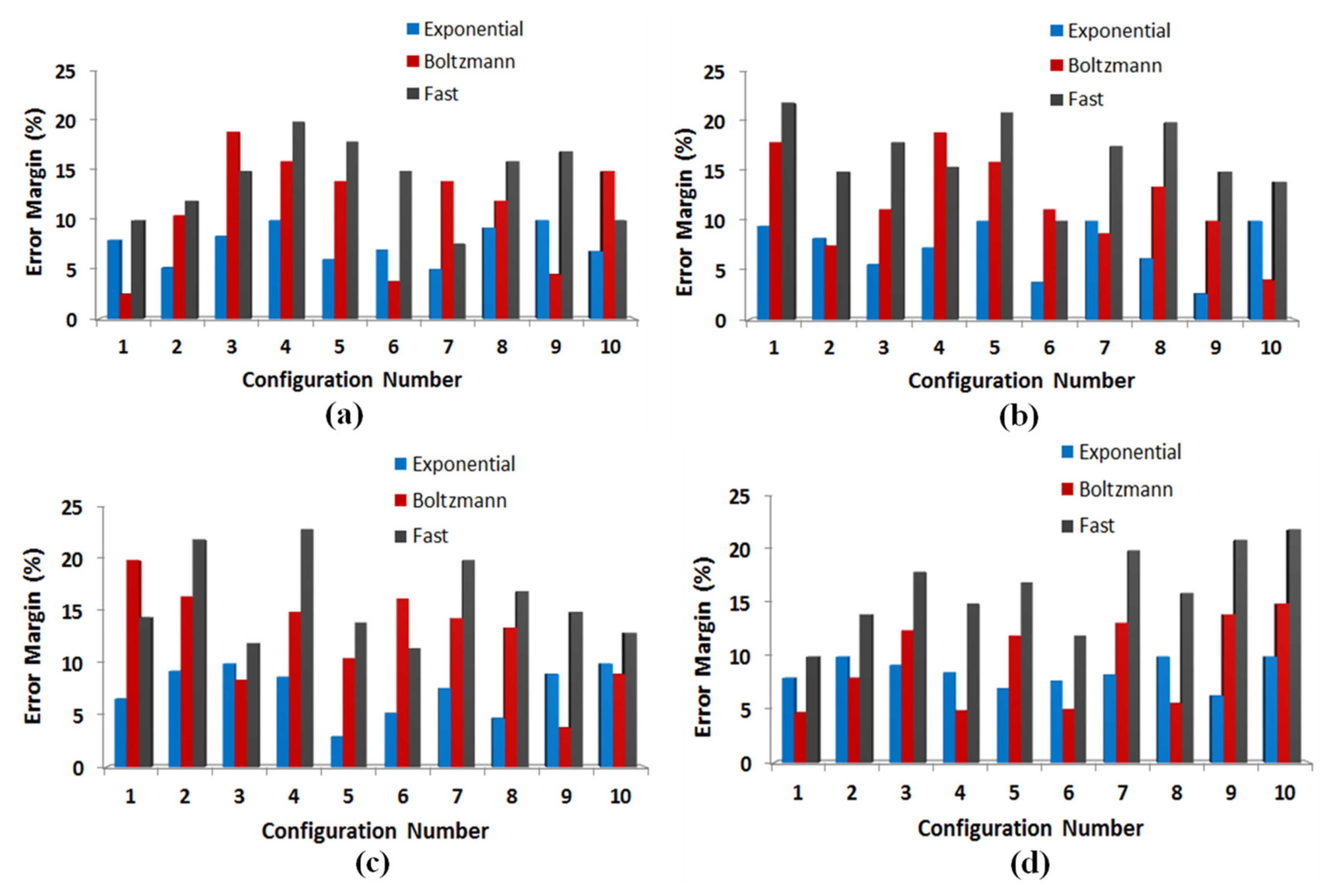
Error margins of the 10 configurations’ layered mediums using exponential, Boltzmann, and fast cooling schedules: (a) chargeability; (b) conductivity at infinite frequency; (c) time constant and (d) exponent term.

Fig. 4

Error margins of the 10 configurations’ objects using exponential, Boltzmann, and fast cooling schedules: (a) chargeability; (b) conductivity at infinite frequency; (c) time constant and (d) the exponent term.

Conversely, fast and Boltzmann cooling schedules yield lower e_m values in some cases when compared to the exponential cooling schedule. However, both of fast and Boltzmann cooling schedules yield worst e_m values that are higher than that for the exponential cooling schedule for an estimated parameter, which could reach values > 20%. According to the results’ analysis, it can be determined that implementing the exponential cooling schedule for the proposed inversion approach yields a reasonably low error percentage for the Cole–Cole estimated parameters when compared with the other two cooling schedules.

V. Conclusion

In this paper, an inversion approach has been presented to estimate the induced polarization information from the electromagnetic fields using information about the electromagnetic source and the scattered electromagnetic data. The proposed approach involves a semi-analytical formulation to perform the forward calculations of the electromagnetic fields that are affected by a polarizable medium. Furthermore, the nonlinear inversion problem is handled using a simulated annealing technique with different cooling schedule designs.

The simulated annealing algorithms were applied to 10 different scatterer configurations to evaluate the effects of the different cooling schedules on the estimated induced polarization parameters. It has been determined that implementing an exponential cooling schedule within the simulated annealing algorithm is the proper inversion scheme to utilize for this problem, given a worst estimation error of about 10%. The obtained results in this research validate the accuracy of the proposed inversion scheme in determining reasonably proper knowledge about the scatterer’s induced polarization properties in light of the non-unique nature of such problems.

Article information Continued