Iterative physical optics (IPO) has been widely used to analyze scattering by large and complex objects, and it iteratively calculates the surface currents on an object based on the magnetic field integral equation and physical optics (PO) approximation [1]. Near-field corrected IPO (NC-IPO) may be an efficient method for this type of computation of an impedance scatterer [2]. The conventional NC-IPO updates the current based on the Jacobi iteration scheme, but other iteration schemes, such as Gauss–Seidel (GS) and successive over-relaxation (SOR), may be more efficient. In [3], an IPO method, along with the GS and SOR schemes, was applied to solve a perfectly electrical conductor (PEC) problem, but the convergence properties of each scheme were not addressed. Therefore, we compare the convergence properties of the Jacobi, GS, and SOR schemes for scattering by several impedance objects.

The conventional IPO update equation, known as the Jacobi iteration, for an impedance object is shown in (1). The IPO update procedure is described in detail in [2].

where R→=r→–r→', R=|R→|, and Jn→ denote the nth-order electric current. k₀, Z₀, Z_s, and n^ denote the free-space wavenumber, impedance, surface impedance, and unit normal vector of the scatterer surface, respectively. The update starts with the zeroth-order PO current, J0→=2n^×Hi→, in the lit region, where Hi→ denotes the incident magnetic field. The Jacobi iteration can be simply represented in terms of an infinite series as follows:

where ∆J→n=Jn→-J→n-1, and the integral terms in (1) can be accurately calculated using the near-field correction (NC) scheme [2].

Because (2) may diverge for a large scatterer, the computation of (2) should be terminated by two stop criteria: the nth residual error (ɛ_n) is less than a given tolerance (δ) and ɛ_n≥ɛ_n–1. The first and second cases pertain to the IPO procedure converging and diverging, respectively. The nth residual error is defined as follows:

During the iteration, the GS scheme directly uses the updated current to calculate ∆J→n. The SOR scheme is a linear combination of Jacobi and GS with a weighting factor w, typically chosen as a value between 0 and 2. For w=1, SOR is reduced to GS.

To investigate the convergence properties of the three linear iteration schemes, five scatterers were considered: boat, vessel, tank, and homogeneous and inhomogeneous aircraft. The five scatterers consisted of the PEC or impedance material. The dimensions, the number of meshes, and the normalized surface impedance (η) of each scatterer are summarized in Table 1, where λ₀ denotes the free-space wavelength. The frequency was fixed at 2 GHz. For the inhomogeneous aircraft, η of the aircraft body, the canopy window, and the radome were 0.39–j0.06, 0.71 – j0.01, and 0.54, respectively. Fig. 1 shows the shape of each scatterer and incident wave direction. The incidence direction and observation line to compute the bistatic radar cross-section were defined by the elevation and azimuth angles, θ_inc and φ_inc, and θ and φ, respectively, which are summarized in Table 2. φ and δ were fixed as 0° and 10⁻³, respectively.

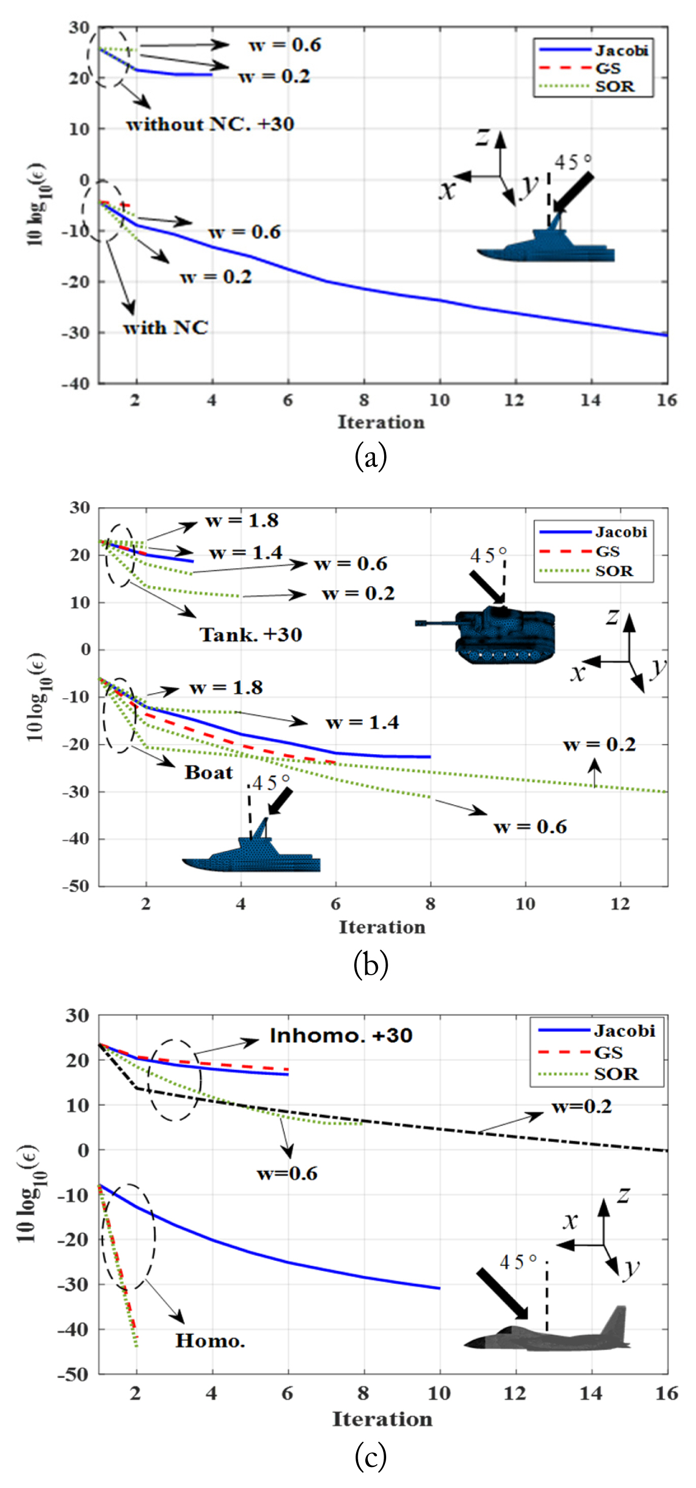
The convergence of the three iteration methods for the PEC boat versus the iteration number is shown in Fig. 1(a). The results of the IPO without the NC scheme were added to 30 for a clear comparison. Owing to the strong interaction among the surfaces, GS without NC and SOR with w = 1.4/1.8, with/without NC, diverge at the first iteration. However, the error of the NC-IPO was slightly less than that of an IPO without NC. For the remainder of the simulation, NC-IPO was used. The SOR weight factor was assumed to be 0.6 if not specified by a number.

Fig. 1(b) and 1(c) show identical comparisons for the impedance boat, tank, and (in)homogeneous aircraft, in which the convergence of SOR with four different weight factors is also compared. The results for the tank and inhomogeneous aircraft were added to 30. Because the reflection by the impedance surface can be less than that by the PEC, more iterations among the surfaces can be calculated for the impedance object, as shown in Fig. 1(b). In addition, the SOR convergence property can be controlled by varying the weight factor; a factor between 0 and 1 can increase the number of iterations. For inhomogeneous aircraft, SOR with a small w of 0.2 can converge to the given tolerance, 10⁻³.

Table 3 summarizes the number of iterations and the normalized root mean squared error (NRMSE) of each iteration scheme for the five PEC or impedance scatterers. In the “# of iterations” row, “D” and “C” indicate the schemes finally diverging and converging, respectively. The NRMSE is calculated as follows:

where σ^MLFMM and σ^IPO are the RCS computed using the multi-level fast multipole method (MLFMM) and IPO methods, respectively. σ^MLFMM is calculated using FEKO. N is the total number of observation points. Notably, GS and SOR can provide an almost identical NRMSE to that of Jacobi at fewer iterations.

Table 4 lists the ratio of the computational time of GS and SOR to that of Jacobi. For this comparison, the ratios for the vessel and tank were omitted because the iteration number was small; therefore, the ratio was almost unity. For this comparison, the tolerance was reduced to 10⁻², which could provide an almost identical NRMSE to that of 10⁻³. GS and SOR can accelerate the IPO convergence speed, particularly for PEC objects.

The convergence properties of three linear iteration schemes were compared for five PEC or impedance scatterers. Among the three schemes, SOR provided an improved convergence property—a smaller number of iterations for the identical error level. In addition, SOR convergence can be controlled by varying the weight factor. Therefore, NC-IPO, in conjunction with the SOR method, could be a robust and efficient scattering analysis method for large-scale scattering problems. Based on the simulations, 0.5 and 10⁻² were initially recommended for the SOR weight factor and tolerance, respectively.