


I. Introduction
As electronic devices are now used in our society, intentional electromagnetic interference can become a threat due to high-power electromagnetic sources. Considering electromagnetic compatibility issues, shielding effectiveness (SE) is an essential factor to investigate the immunity and interference of electronic devices. Especially for personal computers (PCs), SE measurements are necessary because these equipment are commercial devices and do not generally have a high protection level given the surrounding high-intensity electromagnetic field. Recently, Basyigit et al. [1] studied the SE of a PC case and investigated the effects of polarization and aperture dimensions. They used a standard gain horn antenna as a sensor to measure the SE. Although commercial electric field sensors, such as small antennas, D-dot sensors, and electromagnetic wave sensors, are useful tools, there are limitations with respect to their physical sizes and interference of electromagnetic fields to be measured.
Electro-optic (EO) sensors can overcome these limitations for SE measurements. Interference to the electromagnetic field can be minimized because most parts of these sensors consist of dielectric materials and there are no conductive materials for measurements of the field using fiber optic cables. Also, because a size of sensor itself is small (approximately 10 mm), it can be installed in a small space. For several decades, experiments using the EO sensors have been conducted, involving absolute field and SE measurements [2–5] as well as ground penetrating radar applications [6]. These SE measurements [2–4] were conducted in a fully anechoic chamber (FAC) or a semi-anechoic chamber (SAC).
For small conductive enclosures, such as a PC case, three-axis measurements might provide more realistic SE measurements, since the internal electric field would have a totally different polarization with the incident wave due to multiple reflections. Previous works [2, 3, 5, 6] were generally performed using a single axis. Thiele and Geise [4] obtained SE measurements on two axes, they only observed SE values under the condition of a fixed polarization and incident angle.
In this paper, we use the three-axis measurement method to measure the SE of a PC case using EO sensors and observe the effects of the incident angle and polarization of the incident wave in a FAC. We also take the SE measurements in a reverberation chamber (RC).
II. Experimental Method
1. SE of a PC Case
The SE is usually determined by insertion loss measurements, as described in IEEE Standard 299 [7], and is defined by:
where Pref and PDUT are the powers without and with a device under test (DUT), respectively. In our setup, the DUT is a PC case.
For SE measurement in a wide frequency range, a combination of a spectrum analyzer and a tracking signal source can be used for time-efficient measurements. In this paper, we introduce a vector network analyzer (VNA) that is inherently equipped with signal source tracking to a built-in receive module. As a result, the SE can be obtained by measuring the scattering parameters (S-parameters), specifically the transmission coefficient of a two-port network. The magnitude of the transmission coefficient is generally measured in dB by the VNA. The difference of transmission coefficients S21’s in dB between with and without a DUT is defined as the SE of the DUT:
where S21,ref is the transmission coefficient without a DUT, and S21,DUT is the one with the DUT. The relationship between Eqs. (1) and (2) is detailed further in Appendix. The linear magnitude of the transmission coefficient |S21| is converted into S21(dB) using the following equation:
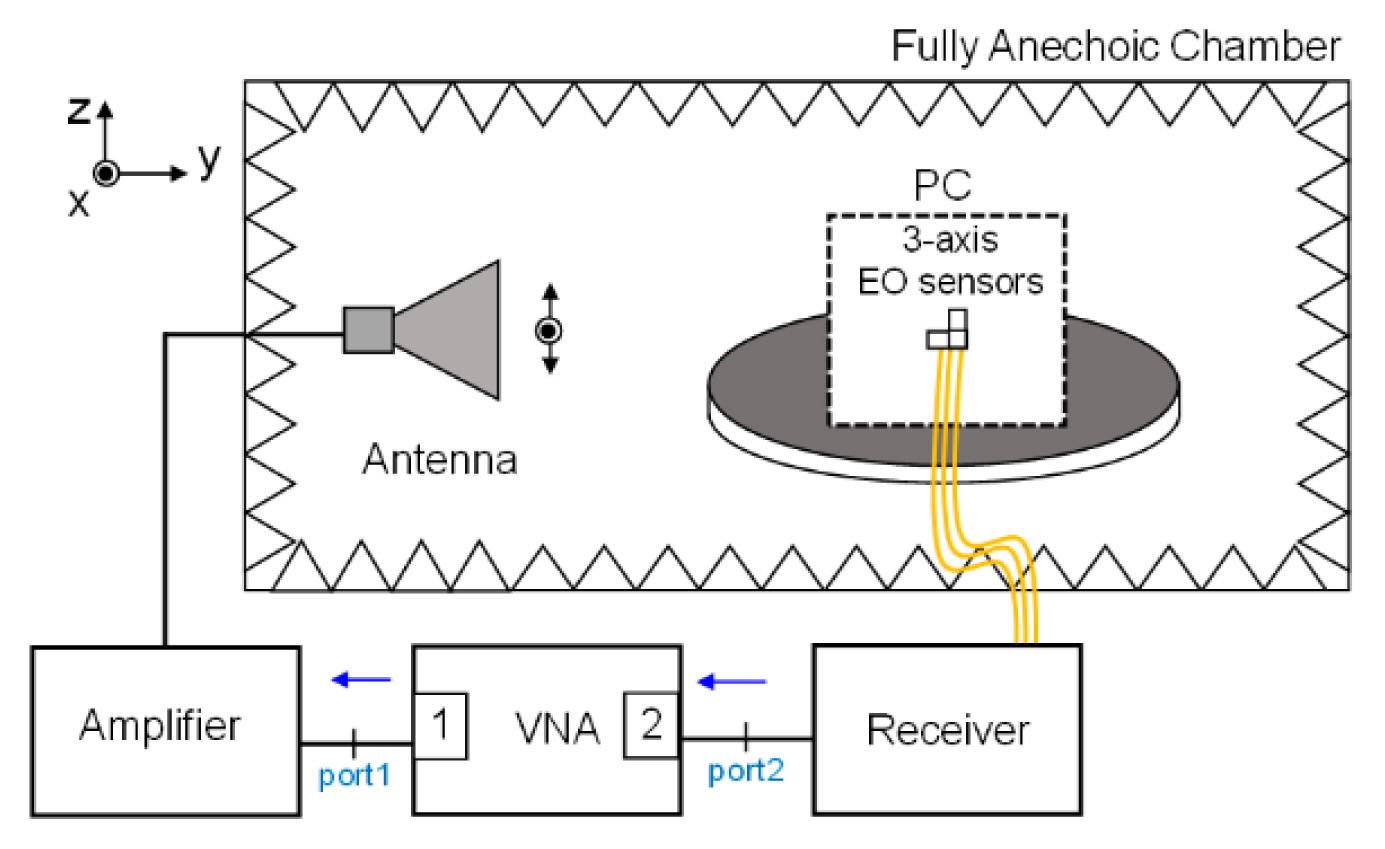
Fig. 1 shows the SE measurement setup. In our configuration, the three-axis EO sensors are placed both with and without the PC case. For the condition of the PC case, the EO sensors are placed at the center of the case. Compared to typical SE measurements, where the axis of the sensor is identical to the polarization of the incident wave, the SE using three axes could give more realistic values because we can observe the internal electric field intensities of the three axes respectively. Therefore, the SEs for the three axes can be described as follows:
Here, S21,ref represents the value of the axis corresponding to the polarization of the incident wave. If the incident wave is vertically (z-axis in our setup) polarized, the S21,ref is considered S21,ref,z.
We also observe the SE of the PC considering all the electric field intensities of the three axes simultaneously as well as separately. To calculate the SE value, the transmitted coefficient S21 in Eq. (2) is substituted, as shown in Eq. (5).
For S21,i (i=x,y,z), the incident voltage to port1 of the VNA is commonly used as the total quantity, accounting for all three axes: V1 = [(V1,x)2 + (V1,y)2 + (V1,z)2]1/2.
2. Measurement Setup in the FAC
The DUT is a PC case (Model: Thermaltake Versa H15) with dimensions 360 mm (L) × 176 mm (W) × 415 mm (H). This PC case includes cables, a main board, and a power supply. A slot hole at the back of the PC case is used to insert the sensors.
Unlike conventional SE measurements based on commercial electric-field sensors, we used a self-developed EO receiver with EO sensors. Most parts of the EO sensor consist of dielectric material, except for its electrode and antenna element.
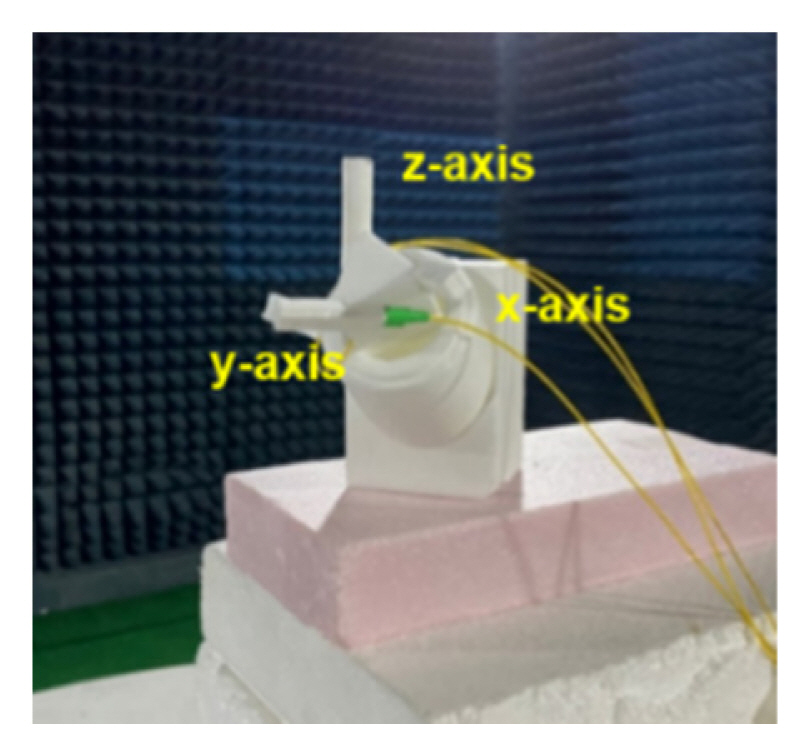
The dimensions for a single axis sensor, including the ROHACELL jig for protection, are 6 mm × 7 mm × 30 mm. To measure the SE for each axis, three sensors are installed in a common mount, as shown in Fig. 2. Due to their small size, the sensors can be placed inside the PC case. The outermost dimension of the three-axis EO sensors is 60 mm × 60 mm × 25 mm.
The SE measurement setup in the FAC is presented in Fig. 1. The PC case is placed on a 0.8-m high wooden round table. A double-ridged horn antenna (ETS, Model 3117) irradiates the PC case. The distance between the case and the antenna is 3 m. The feeding power of port1 of the VNA (Keysight, N9918A) is −5 dBm. The VNA is calibrated at the ends of the cables using the full two-port calibration method with open-short-load (OSL) calibration standards. A 10-W amplifier (AR 10S1G4A) is used to increase the transmitting power. The electric field inside the PC case is measured by the sensors. The sensor is connected to the EO receiver via a 2-m long fiber optic cable. The S21 is measured by the VNA, which utilizes a logarithmic sweep of 601 frequency points and a 100-Hz IF bandwidth.
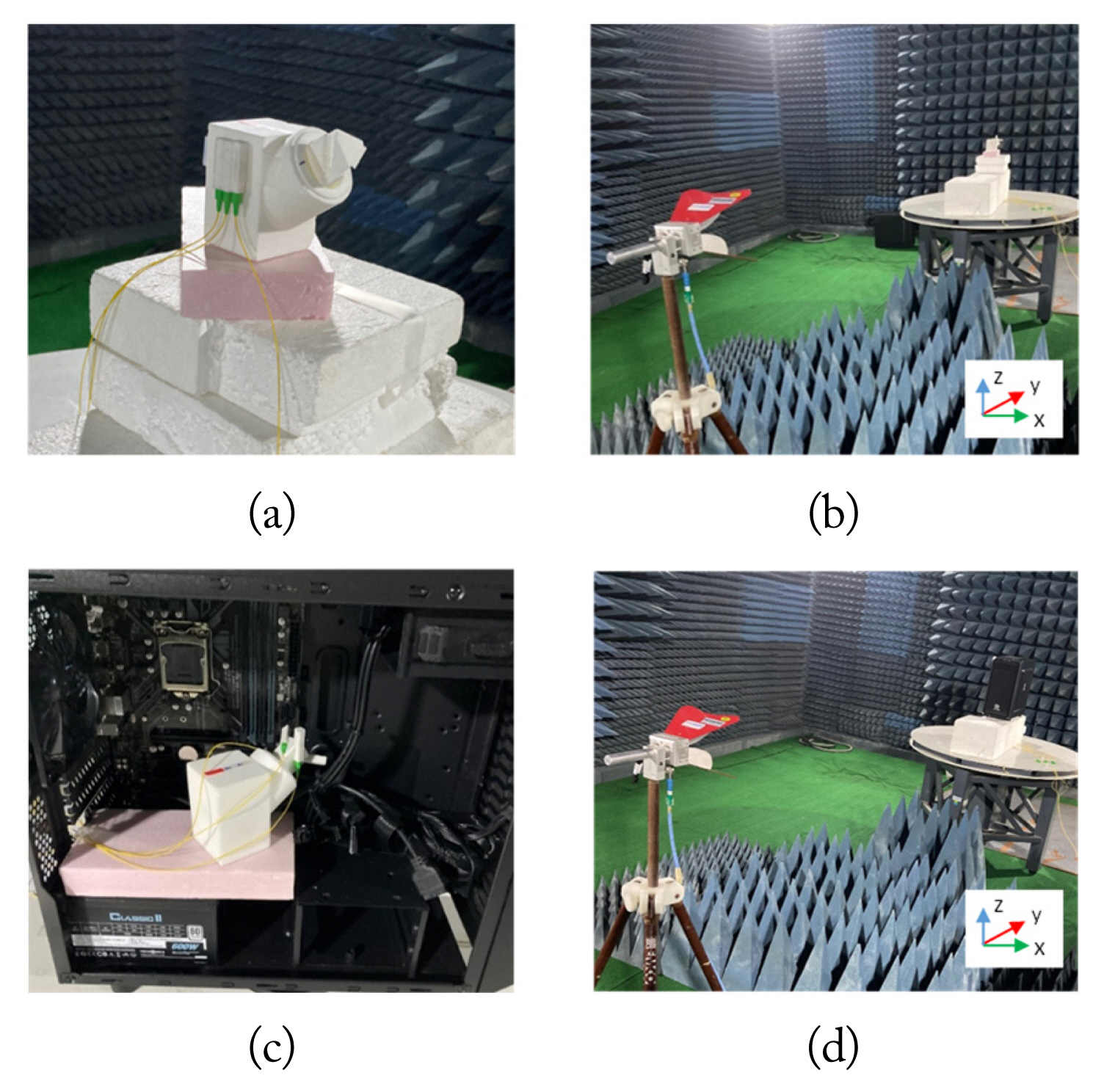
Before conducting the SE measurement, we compared the sensitivities of the three EO sensors in the FAC by measuring S21 under the same conditions as shown in Fig. 3(a). The three sensors are located along the z-axis, which is the same as in the case of vertical polarization.
Next, we performed SE measurements in the FAC to observe the effects of the incident angle and polarization of the incident wave. The antenna is adjusted for the vertical (z-axis) and horizontal (x-axis) polarizations. In addition, the S21 values are measured by azimuthally rotating the PC case from 0° to 180°, with a 45° step.
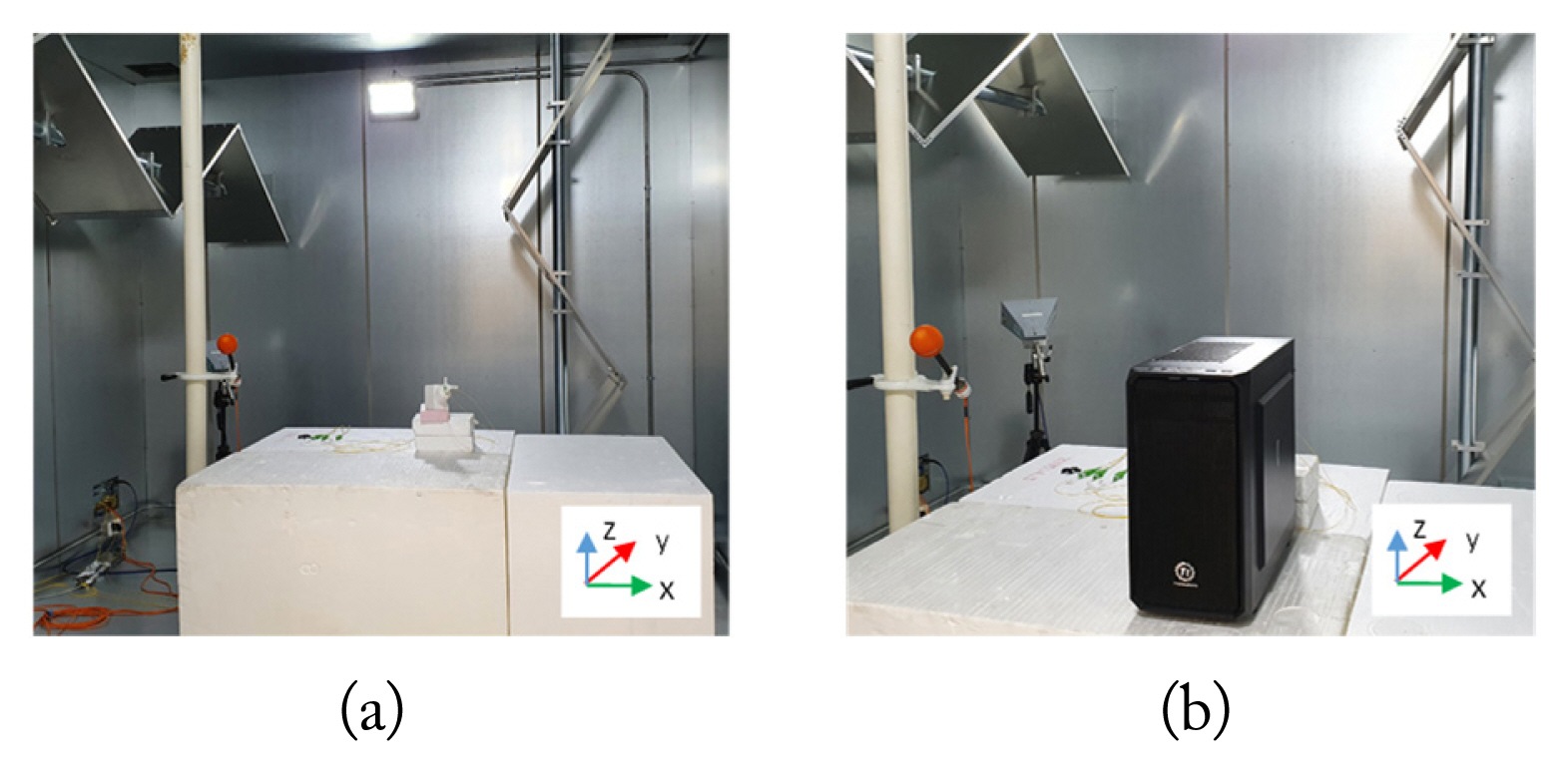
Fig. 3(b) and 3(d) show the experimental setups for the reference- and DUT-measurements, respectively. First, we set a reference position and then measure S21,ref for the three axes in the absence of the PC case. Here, the reference position is the center of the PC case. After the reference-measurement, the sensors are positioned at the center of the PC case (Fig. 3(c)) to measure the S21,DUT parameters for the three axes. Subsequently, the SE values of the PC case are calculated using Eqs. (2) and (4).
3. Measurement Setup in RC
The SE can also be measured in an RC, where electromagnetic waves with all incident angles and polarizations can be efficiently generated. We use a KRISS Reverberation Chamber (KRC) [8] to observe the SE of the PC case. Throughout this process, we can determine the availability of the sensor in the RC.
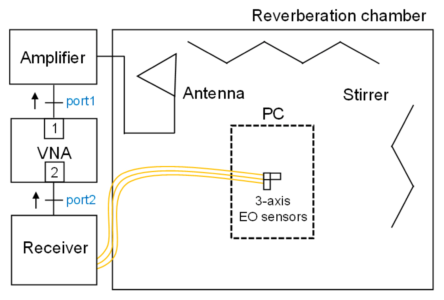
The SE measurement setup in an RC is presented in Fig. 4. The PC case is placed inside a working volume with dimensions 2.2 m (L) × 1.5 m (W) × 1 m (H). As in the case of the FAC, the same amplifier and VNA are used. The output power provided by port1 of the VNA is −5 dBm. The IF-filter bandwidth is set to 1 kHz to reduce measurement time. Furthermore, we experimentally verified that there was no difference in the S21 values between the 100 Hz and 1 kHz IF bandwidths of the VNA in the RC environment. The logarithmic sweep is 601 frequency points. Moreover, since both the horizontal and vertical stirrers are simultaneously rotated from 0° to 330° in a 30° step, we measure the S21,ref and S21,DUT parameters at the center of the PC case. Fig. 5(a) and 5(b) show the experimental setup for the reference- and DUT-measurements, respectively. The sensors are placed on a Styrofoam box. We also placed a three-axis commercial isotropic probe (Amplifier Research, FL7100 & FL7018) at a fixed point in the working volume of the RC to monitor the strength of fields generated in the RC.
III. Characteristics of EO Sensors
The EO sensor implemented in this paper utilizes a folded Mach-Zehnder scheme [9]. A Y-shaped waveguide is installed on an x-cut LiNbO3 substrate and then terminated with a reflective surface. Five segmented electrodes are fabricated on the divided waveguide, which generates an optical path difference when the sensor is exposed to electromagnetic waves.
To activate the EO sensor, we have implemented the EO receiver [10] as depicted in Fig. 6. The receiver contains a laser, a polarization controller, a circulator, and a photodiode. The light from the laser is delivered to the ends of the EO sensor through a programmable polarization controller. The reflected light modulated by the incident electromagnetic wave is demodulated by a photodiode.
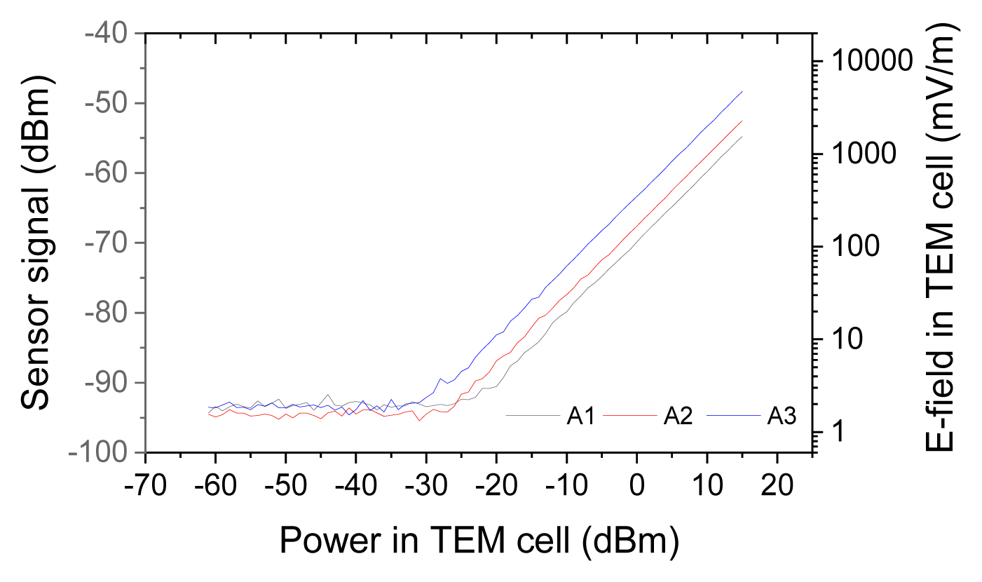
The performance of the EO sensors can be evaluated using a calibration process. The linearity of the three sensors (A1, A2, A3) is presented in Fig. 7. The results are obtained using a TEM cell (IFI, CC-105SEXX), which generates a calculable electric field at arbitrary strength [11], and its upper operation frequency is 1 GHz. The signal emerges from the approximately 2 mV/m level and increases up to 7 V/m.
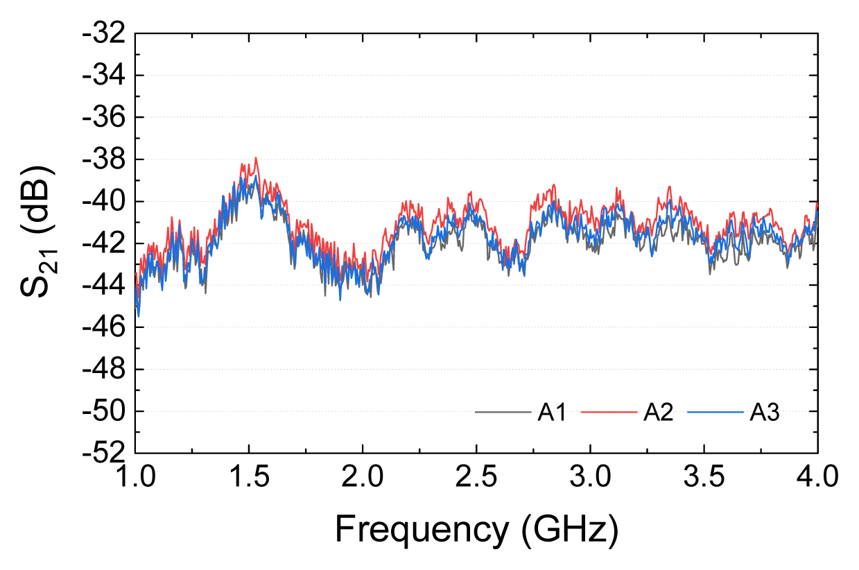
We also compared the sensitivities of the three EO sensors in the FAC by measuring the S21 parameters under identical conditions. The three sensors are located along the z-axis, which is identical to the polarization of the incident wave (Fig. 3(a)). The results of this experiment are shown in Fig. 8.
In Fig. 8, A1, A2, and A3 represent the x-axis, y-axis, and z-axis sensors, respectively. The averaged value from these sensors remains within the range of −40.7 ± 1.5 dB. These results indicate that the performance of the sensors is nearly identical within the frequency range of 1 GHz to 4 GHz. We also find that the sensors exhibit non-flatness in their frequency responses. Presumably, this could be a sensor property as a result of the manufacturing process. In our experiment, the non-flatness of the sensor has no effect on the SE measurements, since the SE here is a ratio of the power levels.
IV. Measurement and Numerical Results
1. SE Simulation
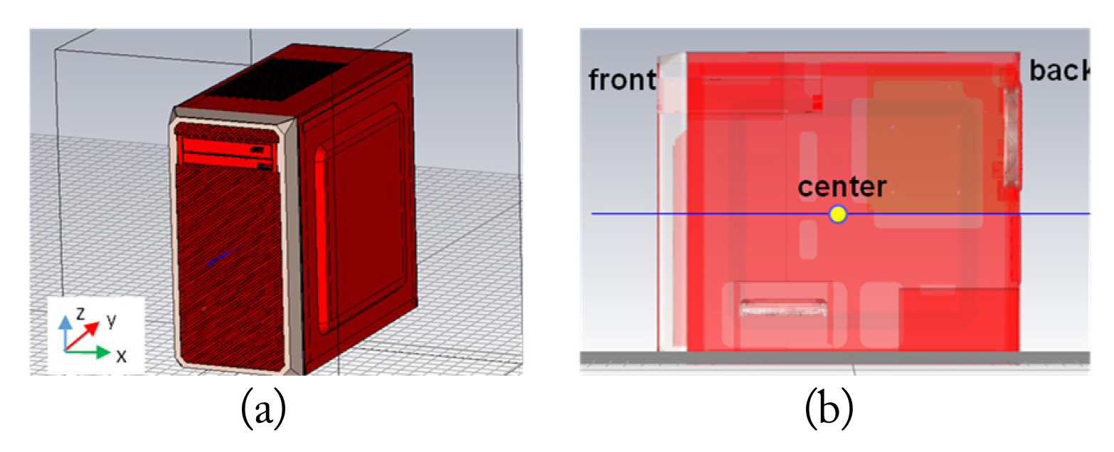
An electromagnetic numerical solver (CST, computer simulating technology) was used for the simulation. Fig. 9(a) presents the simulated PC case model with dimensions of 360 mm (L) × 176 mm (W) × 415 mm (H), which are identical to those of the PC case utilized in our experiments.
In the simulation, the PC case contains a mainboard and a power supply, while cables are neglected to maintain simplicity in the calculation. The material used for the PC parts is iron, except for the front panel, which is made of polycarbonate. The SE values of the PC case for the incident angle and polarization are calculated by considering the experimental conditions. The frequency range in the simulation is set at 1 GHz to 4 GHz. A simulating probe is placed at the center of the enclosures, as shown in Fig. 9(b).
2. Measurement and Numerical Results in the FAC
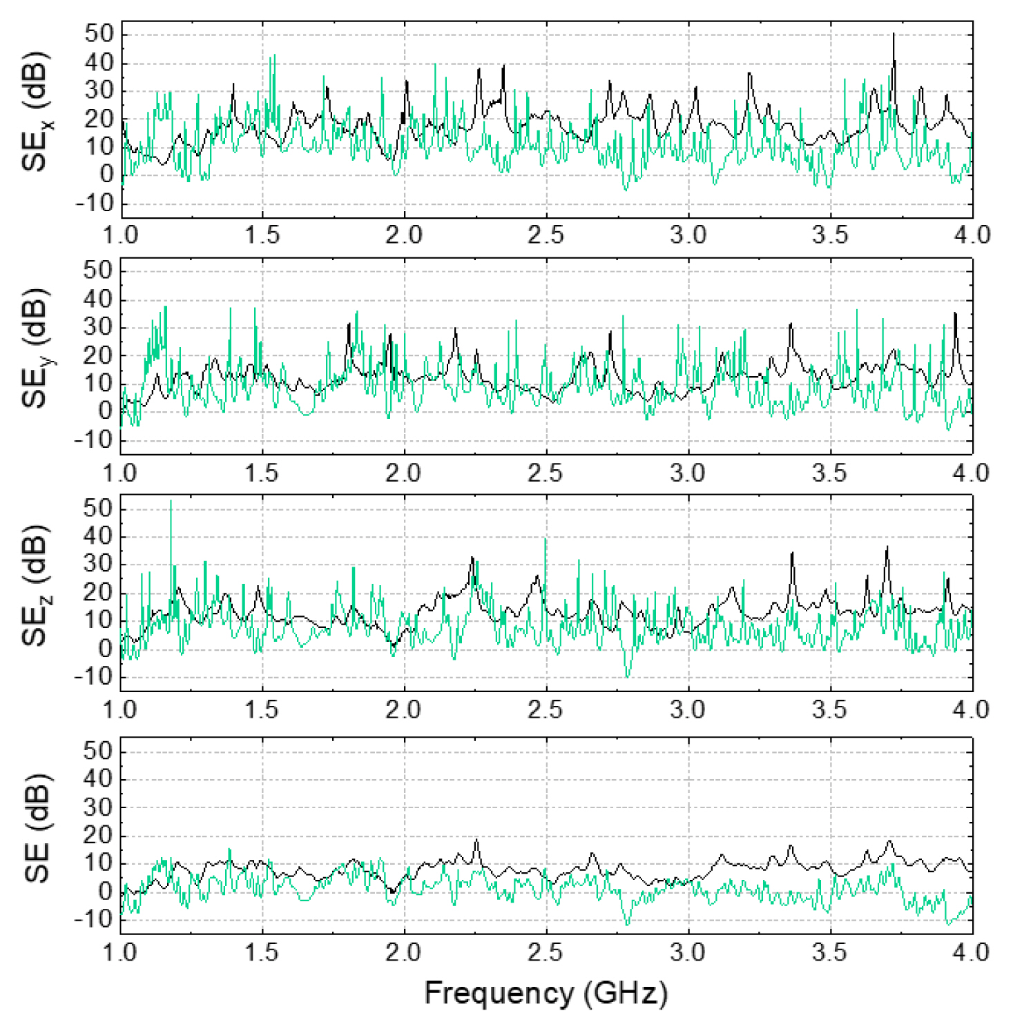
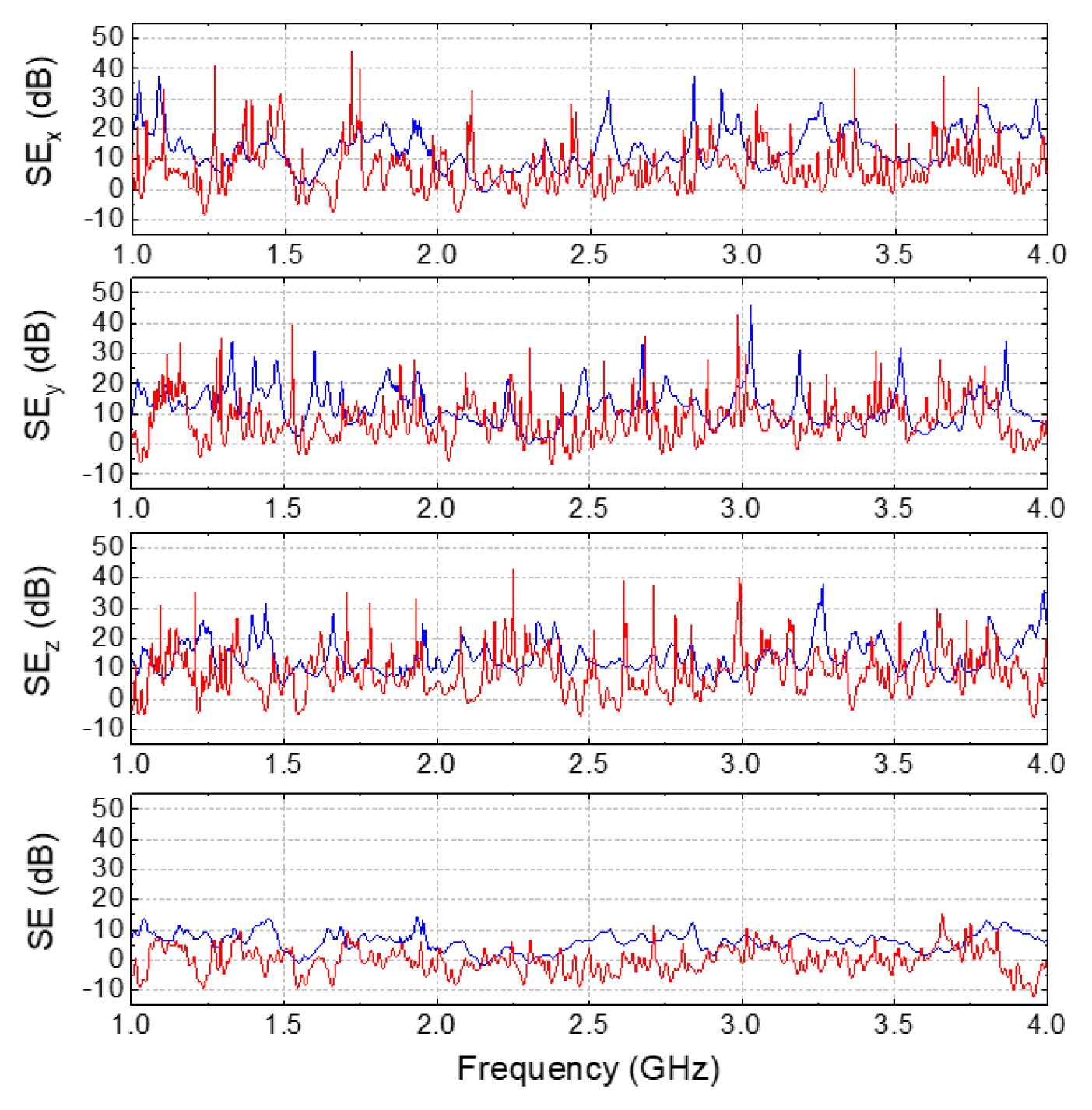
To measure and simulate the SE of the PC case for the individual axes, the sensors or probes are first placed at the center of the case, with the incident angle being 0°. Fig. 10 shows the SE values for vertical polarization. The black and green lines represent the measured and simulated results, respectively. Fig. 11 shows the SE values for horizontal polarization. The blue and red lines represent the measured and simulated results, respectively.
While the incident wave is vertically (z-axis) or horizontally (x-axis) polarized, the transmitted wave inside the PC case has a totally different polarization because of the multiple reflections in such a case. For each axis, the SE value shows a different pattern.
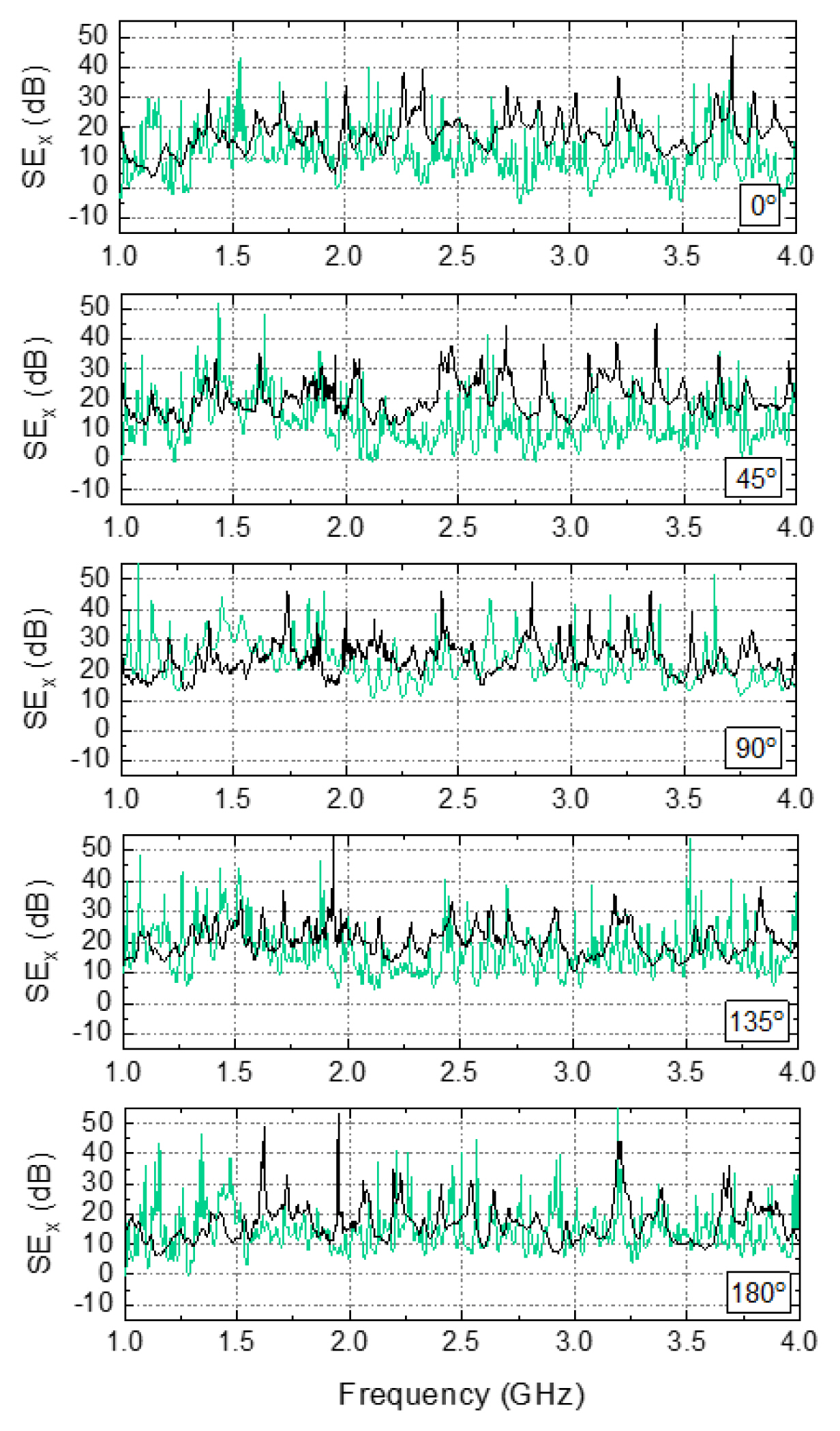
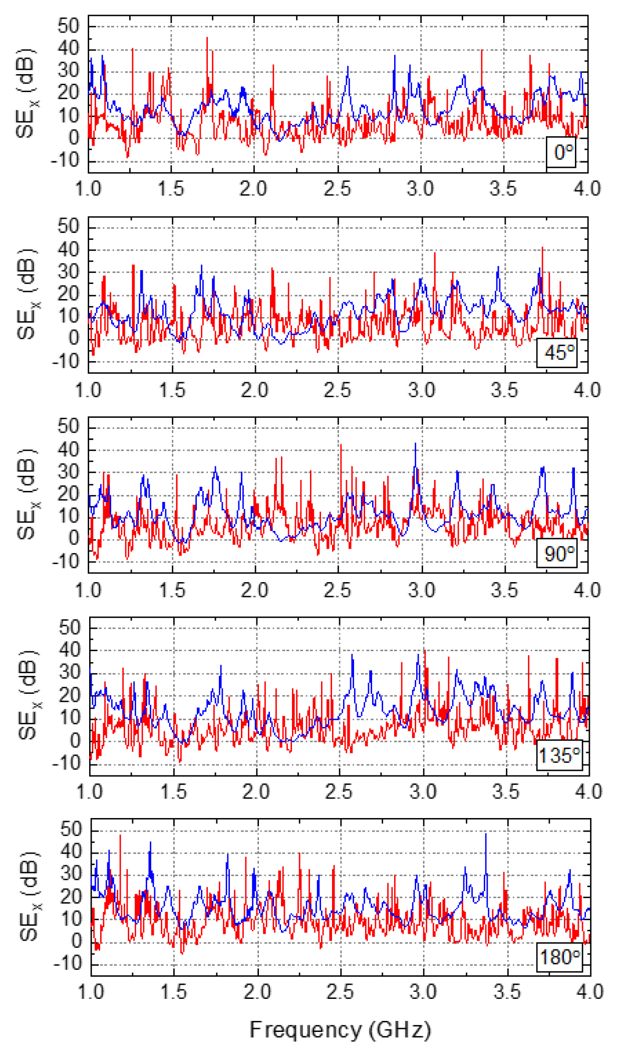
We also measure and simulate the SEx of the PC case at the center as a function of the incident angle. Fig. 12 shows SEx for vertical polarization. The black and green lines represent the measured and simulated results, respectively. Fig. 13 presents the SEx for horizontal polarization. The blue and red lines represent the measured and simulated results, respectively.
These results indicate that the SE in the numerical simulation has more peaks than in the experiments. The discrepancy between the two results could be a result of the FAC environment and imperfect conditions in the simulation. Even though the number of data points in the simulation is larger than in the experiment, the number of data points has little effect on the frequency-dependant tendency of the SE but increases noise signals.
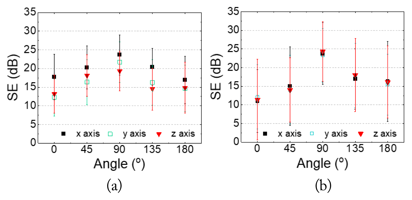
To clearly observe the effect of the incident angles, the average values with the error bars of the SEx, SEy, and SEz for both the vertical and horizontal polarizations are calculated, as presented in Figs. 14 and 15, respectively. The error bars represent the standard deviations of SEx, SEy, and SEz over the frequency range. The results show no significant difference between the measurement and simulation results.
We also find that the incident angles have different effects according to vertical and horizontal polarization. For vertical polarization, the SE values exhibit dependence on the incident angle. The measured SE has the peak value at an angle of 90°, with the incident wave irradiating the right side of the PC case, which has no holes at the same angle. Unlike vertical polarization, the SE values for horizontal polarization are within the error bars for all incident angles.
3. Measurement Results in the RC
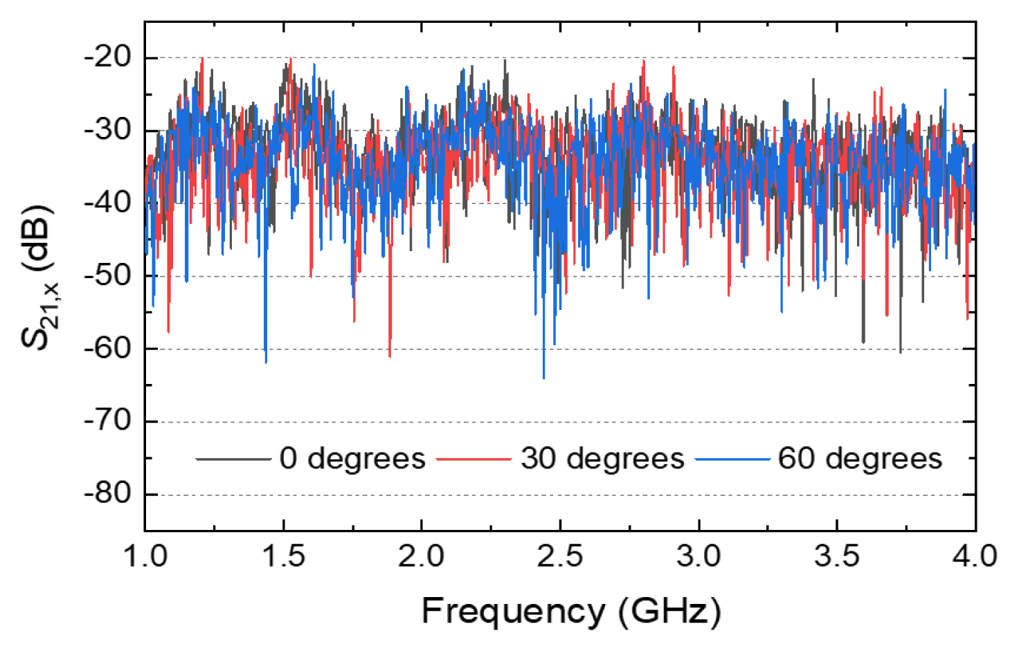
This section describes the procedure for calculating the SE values in the RC. First, we sequentially measure S21,x, S21,y, and S21,z as the reference-measurements. Since the horizontal and vertical stirrers are rotated simultaneously from 0° to 330° by a 30° step, we can obtain twelve S21 values for each axis. Fig. 16 shows the S21,x value for the reference-measurement. Here, we present the S21,x for three angles, since the S21,x for the other rotation angles of the stirrers have a similar pattern. Next, we calculate |S21,ref| by using Eq. (5).
where j denotes a number corresponding to the stirrer angle. Then, we also measure S21,x, S21,y, and S21,z as the DUT-measurements [12]. The |S21,DUT,i| for each axis and the |S21,DUT| considering the three axes simultaneously can be reduced by Eq. (7) and Eq. (8), respectively. Finally, we can obtain the SE values using Eqs. (2) and (4).
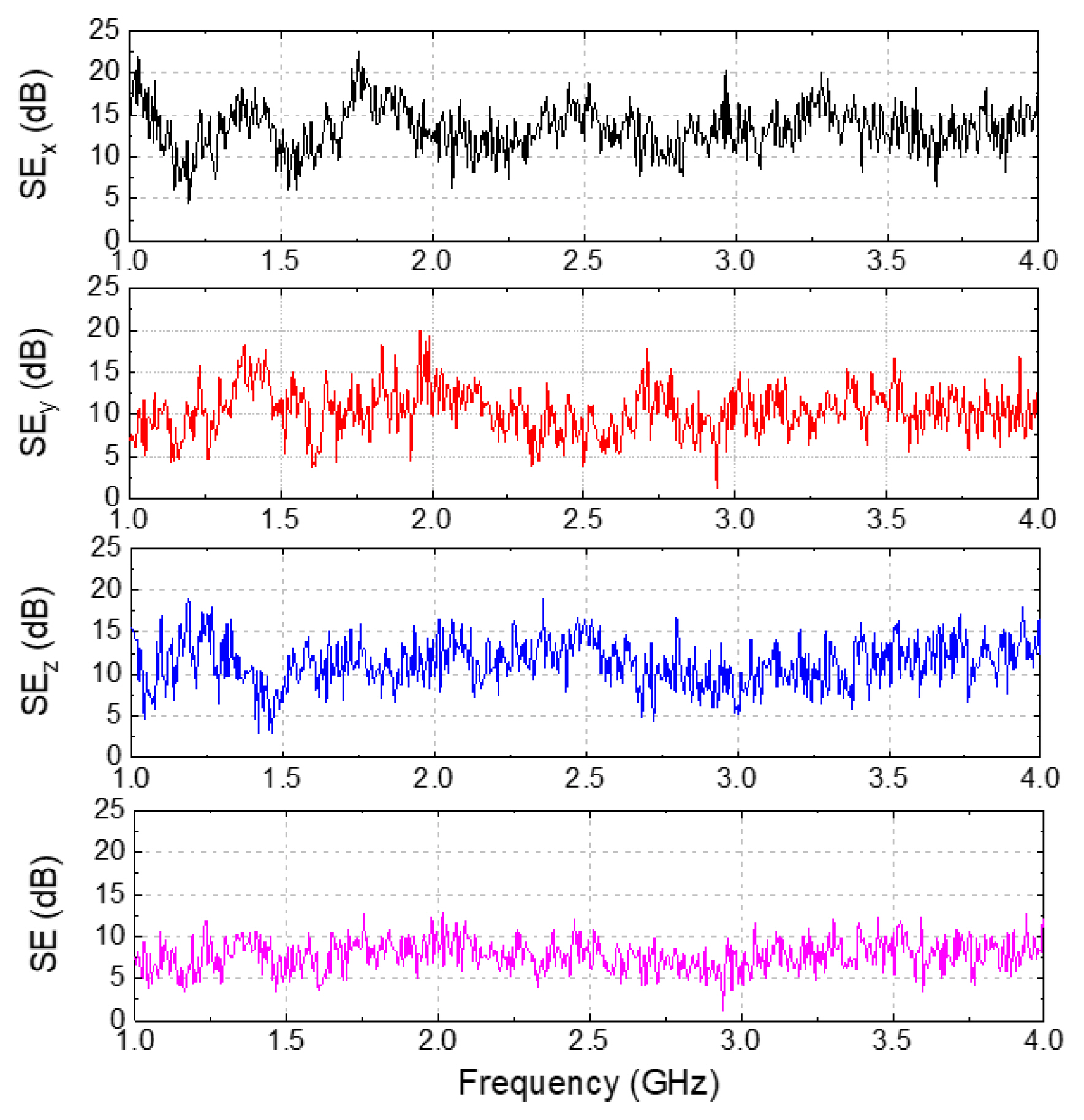
Fig. 17 shows the measured SE values at the center of the PC case in the RC system. From the results, we can find how the incident wave is transmitted into the PC case and polarized for each axis. Also, the measured results show more variation in the frequency domain than in the case of the FAC because all incident angles and polarizations exist simultaneously in the RC. The average values over the frequency range for the SEx, SEy, and SEz are 13.4 ± 2.8 dB, 10.4 ± 2.8 dB, and 11.3 ± 2.8 dB, respectively. The average value for SE considering the three axes simultaneously is 7.6 ± 2.1 dB. These measurements also confirm that the SE measurement of the PC case using an EO receiver system is feasible for an RC system.
V. Discussion and Conclusion
We present the SE measurements of a PC case using three EO sensors (x-, y-, and z-axes) in a FAC and an RC system. The frequency range is from 1 GHz to 4 GHz.
In the case of the FAC, we analyzed the effects on the SE of the PC case according to the incident angle and polarization in our frequency measurement range. We also used the computer simulation software CST to obtain numerical results, which were then compared to the experimental results. Although the SE values of the numerical and experimental results over the frequency range exhibited discrepancies, the average values of the SE in both results showed a similar trend with an approximate 6 dB error. These findings indicate that this simulation will be helpful for predicting averaged SE values. In the case of the RC, we measured the SE values for each axis.
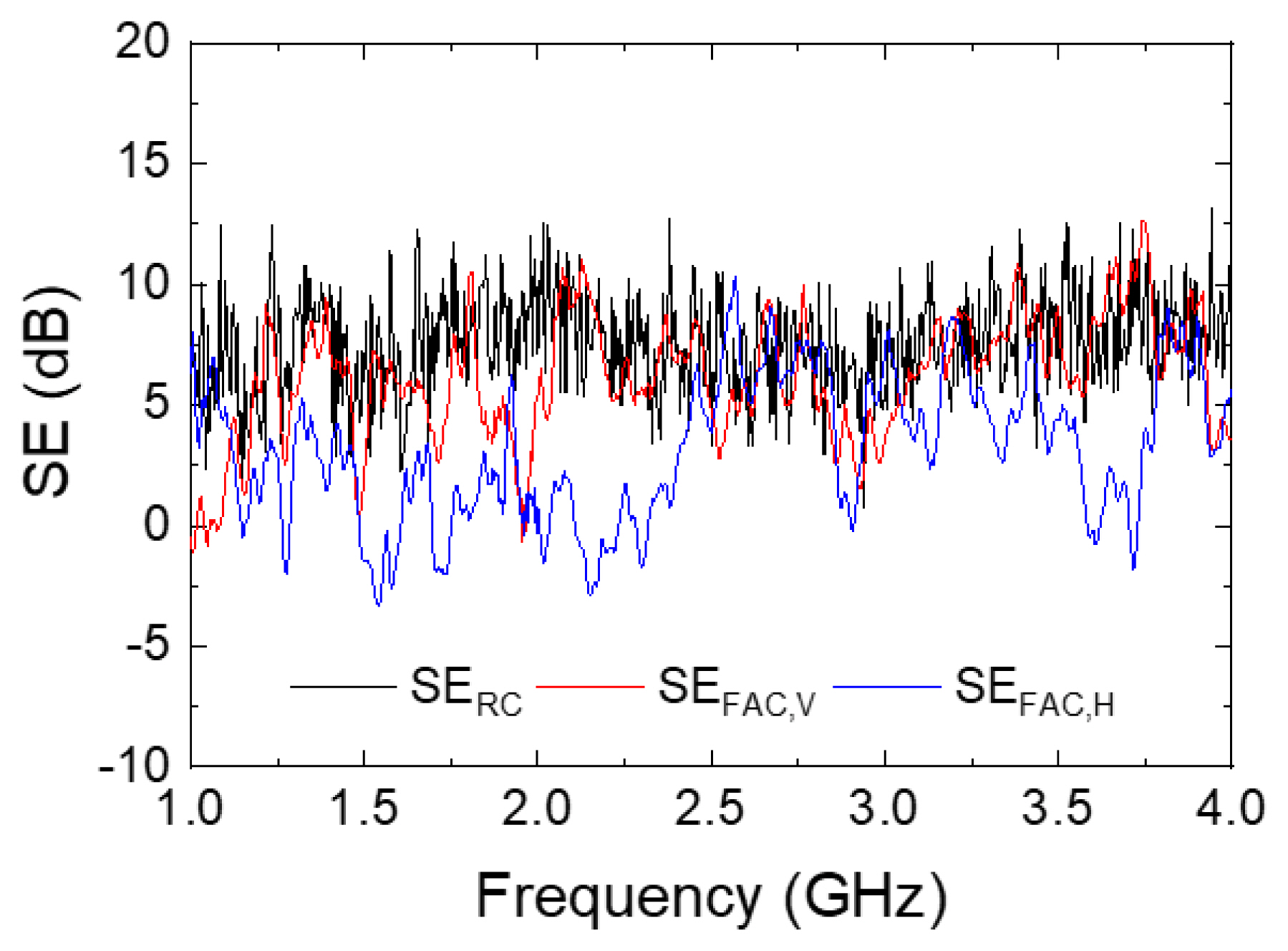
Fig. 18 shows the SE values of the PC case considering the three axes simultaneously for both the FAC and RC systems. The SEFAC,V and SEFAC,H according to the incident angle for the vertical and horizontal polarizations are 6.2 ± 2.6 dB and 3.2 ± 3.0 dB, respectively, as calculated from the experimental results. In the case of the RC, the SERC for the center of the PC case is 7.6 ± 2.1 dB.
These results indicate that the EO receiver system implemented in this paper can be applied to SE measurements in both FAC and RC systems. Moreover, SE values ranging from 1 GHz to 4 GHz for a single measurement are obtained by utilizing a VNA and a 10-W amplifier based on EO sensors. We believe that our measurement technique based on EO sensors and a VNA will contribute to the further development of efficient and reliable SE measurement methods for enclosures.