


I. Introduction
When hypersonic vehicles enter the atmosphere, the communication blackout problem occurs because of the dusty plasma sheath phenomenon [1]. Experimental research on electromagnetic (EM) wave propagation in dusty plasma is expensive and time consuming due to the high-temperature condition requirement. Alternatively, numerical research is promising to systematically analyze EM wave propagation in dusty plasma with various parameter conditions. The finite-difference time-domain (FDTD) method has been widely used to analyze EM wave interaction with complex media [2–6] due to its simplicity, robustness, and accuracy [7–11]. In a previous work [12], we proposed the FDTD formulation to be suitable for time-invariant dusty plasma by utilizing a bilinear transform (BT). For time-invariant dusty plasma, the BT-FDTD simulation was 2.64% faster than the conventional shift operator (SO)-FDTD formulation, with less memory requirements and the same numerical accuracy.
The electron density of dusty plasma changes with time [1, 13, 14]. Therefore, the time-varying characteristics of dusty plasma should be considered to accurately analyze EM wave propagation in dusty plasma. Note that time-varying coefficients should be updated every FDTD time marching in the FDTD formulations of time-varying media. In this work, we propose an efficient FDTD modeling suitable for time-varying dusty plasma. For this purpose, we first extend BT to the FDTD formulation of time-varying dusty plasma. A higher speedup of the BT-FDTD formulation versus the SO-FDTD formulation can be achieved for the time-varying dusty plasma than for the time-invariant case because fewer arithmetic operations are involved in updating time-varying coefficients in the BT-FDTD formulation. Moreover, the state-space approach is applied to the BT-and SO-FDTD formulations because it can reduce the memory requirement of dispersive FDTD formulations [15–17]. We apply the state-space approach to reduce the computation time and memory requirement in the BT-FDTD formulation for time-varying dusty plasma. Numerical examples illustrate that the proposed FDTD simulation is 118.63% faster than its SO-FDTD counterpart, albeit with the same computational accuracy and less memory usage.
II. FDTD Formulation for Time-Varying Dusty Plasma
In real dusty plasma, all parameters are time-invariant, except for electron density [13, 14]. The time-varying electron density Ne is defined as follows:
Here, f(t) represents the time-varying function, and Ne,0 is the constant of the electron density. The time-varying characteristic of electron density affects two dusty parameters. Therefore, angular plasma frequency
ω p e 2 ( = N e e 2 / ɛ 0 m e ) η e d ( = e 2 π r d 2 N e N d / m e )
where ωpe,0 and ηed,0 are the constants of the angular plasma frequency and the charging response factor, respectively. In the equations above, ɛ0 is the permittivity of free space, e is the electric charge of an electron, me is the mass of an electron, rd is the radius of dust particles, and Nd is the density of dust particles. Note that other dusty parameters are time invariant.
In the following subsections, we first briefly discuss the conventional SO-FDTD formulation for time-varying dusty plasma and then address the extension of the state-space approach. We then propose an efficient BT-FDTD formulation with the state-space approach, which is highly suitable for time-varying dusty plasma, and present a comparison of computational efficiency for the SO- and BT-FDTD formulations.
1. SO-FDTD
The dispersion relative permittivity model of dusty plasma in the frequency domain can be expressed as [15]
where ɛr,∞ is relative permittivity at an infinite frequency, c0 is the speed of light in free space, νch is the dust charging frequency, and νeff is the effective collision frequency.
In the frequency domain, Maxwell’s curl equations and the constitutive equation can be written as follows:
The time-domain governing equations are obtained by applying the inverse Fourier transform. The update equations for SO-FDTD can be derived by applying the central difference scheme (CDS) to the resulting Maxwell’s curl equations and the SO approach to the time-domain constitutive equation.
where
with
Here, the superscript indicates the FDTD time index, and Δt represents the FDTD time step size. The update coefficients Ba–Bd are the functions of time, and they can be rewritten by decomposing the time-varying and the time-invariant parts. For example, Ba is expressed as
In actual FDTD simulations, the update coefficients are usually pre-calculated before the FDTD time marching to speed up the computation time. However, for the FDTD formulation of time-varying dusty plasma, the time-varying coefficients should be updated for each FDTD time loop. In Eq. (10), many field components on the right-hand side are included, which leads to a large memory requirement.
In this work, the state-space approach [16–18] is employed to reduce memory usage. In the state-space approach, field variables at the same time step are assigned to a new alternative variable. For example, the update equation for E in Eq. (10) can be written as
(11)
The variable W1 represents the grouped field variables at the time step n in Eq. (10), and W2 and W3 represent the variables at n–1 and n–2, respectively. Note that five field components are required in the SO-FDTD method with the state-space technique, while seven field components are needed in the standard SO-FDTD method.
2. BT-FDTD
Here, we discuss an efficient FDTD modeling for the EM analysis of time-varying dusty plasma. In our previous work [12], the computational efficiency of the BT-FDTD formulation was better than that of the SO-FDTD formulation for the EM analysis of time-invariant dusty plasma. In the current work, we propose the FDTD modeling to be highly suitable for time-varying dusty plasma by utilizing both the BT and the state-space approach.
In BT-FDTD, Ampere’s equation and the constitutive equation in the frequency domain are expressed as follows:
with
The FDTD update equation of E can be obtained by applying the inverse Fourier transform to Eq. (12) and then the CDS to the resulting equation:
where ɛ∞=ɛ0ɛr,∞. The FDTD update for J is derived by utilizing the BT approach to Eq. (13):
Note that in the BT approach, jω is approximated as
In the above equations, the coefficients are as follows:
with
It is worth noting that only multiplication is involved in the time-varying coefficients, unlike in the SO-FDTD formulation, in which addition and multiplication are required. The FDTD update equation for H is the same as that for SO-FDTD. As the En+1 field in Eq. (14) cannot be updated explicitly, we plug Eq. (15) into Eq. (14).
The resulting FDTD update equation for E is expressed as follows:
(17)
Three coefficients are functions of time in the proposed BT-FDTD formulation, while four coefficients are time varying in the SO-FDTD formulation.
We then apply the state-space approach to the BT-FDTD method. The FDTD update equation for J can be expressed as follows:
Comparing the above update equation with Eq. (15), one field variable is less required by applying the state-space technique.
Note that unlike SO-FDTD, BT-FDTD can further simplify the E field update equation by using the state-space approach. In Eq. (17), we can replace the variables at time step n–1 in
W 2 n + 1
By using Eq. (19), we can simplify the above equation as follows:
In this additional manipulation, the complexity of the E field update equation of BT-FDTD is drastically reduced, enhancing the computational efficiency of BT-FDTD.
Table 1 shows the memory requirement and the number of arithmetic operations of the SO-FDTD and BT-FDTD formulations for time-varying dusty plasma. Here, A/S indicates addition/subtraction, and M/D indicates multiplication/division. Note that the arithmetic operations for the time-varying update coefficients are included in this table. In the table, we consider the standard FDTD method (without the state-space approach) and the FDTD method with the state-space approach. The memory requirement for the BT-FDTD formulation is less than that for the SO-FDTD formulation, regardless of whether the state-space approach is applied. In addition, the BT-FDTD formulation with the state-space approach is significantly better than the SO-FDTD formulation in terms of computation time (related to the number of arithmetic operations). It should be noted that in the EM analysis of time-varying dusty plasma, the state-space technique is more appropriate for the BT-FDTD formulation than for the SO-FDTD formulation with respect to computation time because it can be efficiently used in two FDTD update equations of the former formulation but only in one update equation of the latter. Table 2 presents the details of the computational efficiency of the FDTD formulations with the state-space approach. Additional operations are required for time-varying characteristics. More A/S operations are not required in the BT-FDTD formulation compared to SO-FDTD, thus implying better computational efficiency of the former than the latter.
III. Numerical Examples
We investigate the computational efficiency and accuracy of the SO-FDTD and BT-FDTD formulations. We use one-dimensional inhomogeneous dusty plasma with a thickness of 0.15 m and 30 slabs with different Ne, following [14]. The other dusty plasma parameters are Nd = 1012 m3, νeff = 10 GHz, and νch = 8.7 GHz. The simulation frequency range is 1–100 GHz. We define the FDTD space step size as Δz = 40 μm and the FDTD time step size as Δt =0.125 ps. The computational domain is terminated by 10-cell perfectly matched layers [19–21]. All FDTD simulations are performed using an Intel i7-10700 CPU.
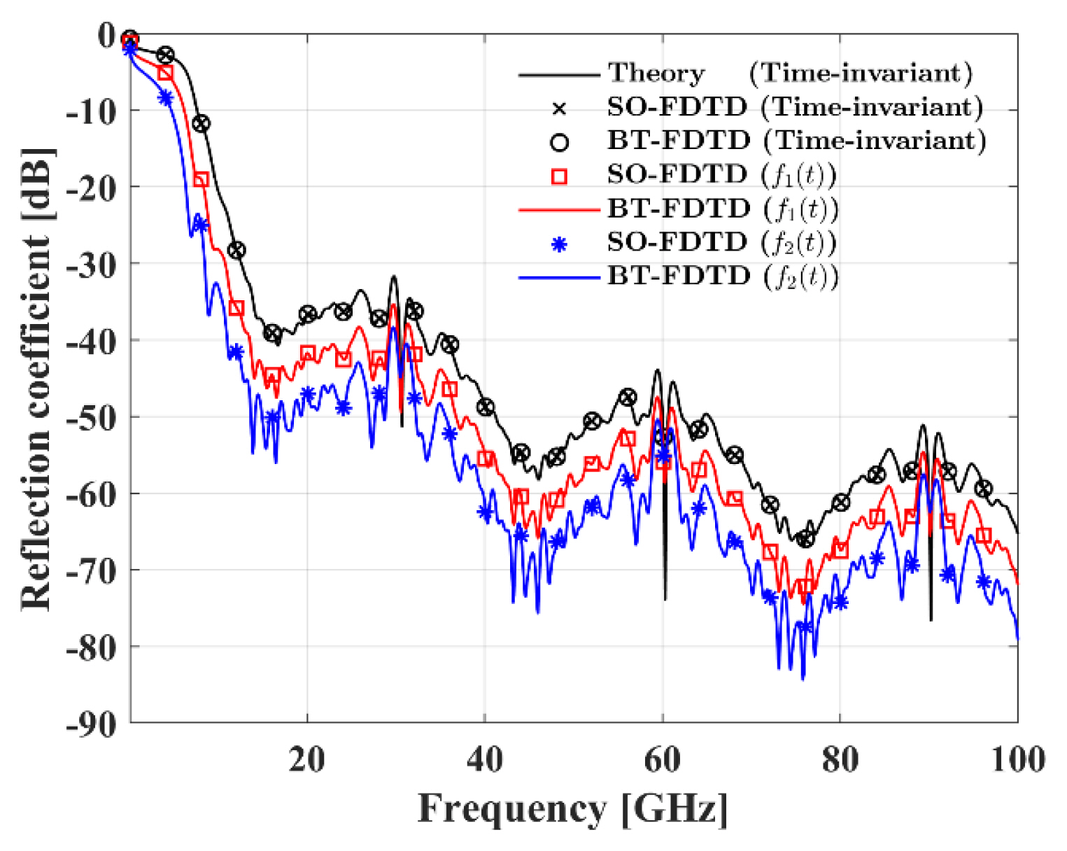
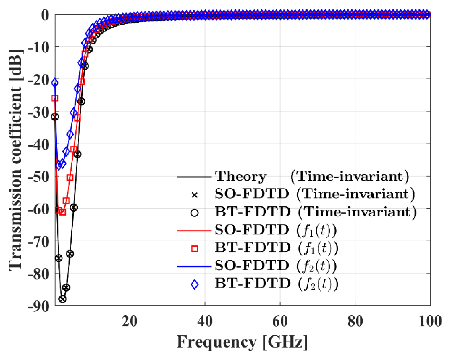
Time-invariant dusty plasma is analyzed by setting f(t) to validate our FDTD simulations. As shown in Figs. 1 and 2, both FDTD simulations agree well with [22]. We then simulate the FDTD formulations with the state-space approach for time-varying dusty plasma. In this work, two time-varying functions are considered:
f 1 ( t ) = t / T r
We then compare the computation time and memory cost of FDTD simulations (with and without the state-space approach) for time-varying dusty plasma. As shown in Table 3, the computational efficiency of the BT-FDTD formulation is better than that of the SO-FDTD formulation. For the standard FDTD method (without the state-space approach), the BT-FDTD simulation is 3.7% faster than the SO-FDTD simulation. However, the BT-FDTD formulation with the state-space approach is approximately 118.63% faster than the SO-FDTD formulation. For time-invariant dust plasma, the BT-FDTD simulation is 2.64% faster than the SO-FDTD simulation [12]. Moreover, less memory cost is required for the BT-FDTD simulations than for the SO-FDTD simulations.
IV. Conclusion
In this work, we propose an efficient FDTD formulation for EM wave propagation in time-varying dusty plasma using the BT technique and the state-space approach. BT-FDTD is more adaptable to time-varying dusty plasma than SO-FDTD. Moreover, the state-space approach is more effective for the proposed BT-FDTD formulation than for the SO-FDTD formulation in the EM analysis of time-varying dusty plasma. We apply the state-space approach to the J field update equation of BT-FDTD by grouping the variables at the same time step as the W variables. We optimize the E field update equation of BT-FDTD using the defined W variables. As a result, the FDTD update formulation of BT-FDTD is much simpler than that of SO-FDTD and has better computational efficiency in time and memory, with the same accuracy. Numerical examples are used to validate the computational efficiency improvement in the proposed FDTD modeling of time-varying dusty plasma. The proposed FDTD modeling approach using the combination of BT and the state-space approach can be extended to other time-varying dispersive media in nanophotonics and metamaterials.