


I. Introduction
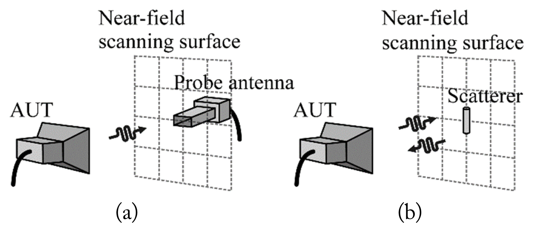
To measure the radiation pattern of an antenna, a two-port measurement system is usually considered. In the two-port measurement system, the antenna under test (AUT) is driven by a known source, and the probe antenna, which is located in the far zone of the AUT, measures the radiation intensity. The radiation pattern of the AUT is obtained directly by tabulating the measured radiation intensity and the angular location of the probe [1]. In millimeter-wave bands, the antenna systems are packaged such that it is difficult to disassemble. If it is necessary to disconnect the radiator antenna from the driving circuitry to measure the radiation pattern, it is difficult to drive the antenna and the radiation characteristics of the antenna would change. In such cases, an indirect antenna measurement technique needs to be considered.
Many antenna systems are electrically large if the mounting platform is included [2, 3]. In such cases, a long distance is required to meet the far zone criteria. In some cases, it may be practically impossible to secure the required distance. Therefore, in this paper, a novel antenna measurement technique is proposed. In the proposed technique, the radiation characteristics are measured using a scatterer that scans in the near-field of the AUT, as shown in Fig. 1. The scattered field is measured by the AUT itself, and the measured quantity is transformed to the farfield pattern using a near-field to far-field transformation (NTFT) method that is proposed in this paper for the one-port measurement method. The proposed measurement technique is advantageous over two-port systems in many aspects. The system hardware configuration is simple. The scatterer can be made light weight and, thus, the scanning is easy. There are no moving cables, and the distortion due to the cable can be minimized. Scatterer-based systems have previously been studied [4ŌĆō6]. However, [4] is only focused on electric field data acquisition, [5] is valid for obtaining a single-plane radiation pattern for linear-polarization and simple aperture antennas, and [6] requires other modulation systems.
In general, the measurement accuracy can be improved by the probe compensation method in a two-port measurement system [7]. Similarly, by compensating the characteristics of the scatterer, the accuracy of the one-port measurement system could be improved. In this paper, a scatterer compensation method for one-port planar NTFT is derived based on the reciprocity theorem. The proposed compensation method is validated through experiment.
II. One-Port Near-Field Antenna Measurement Setup
When two antennas are in the far zone of each other, the relationship between the power received by one antenna and the power transmitted by the other antenna can be simply described by the Friis transmission equation [1]. For the case that each antenna is matched to their respective feeding circuit, the equation can be written as:
where Gt and Gr are the gains of the antennas, Žü╠ét and Žü╠ér are polarization unit vectors of the transmitting and receiving antennas, respectively, ╬╗ is the wavelength, and R is the distance between the two antennas. If we use a two-port measurement system, such as a network analyzer, |S21|2 may be proportional to the power ratio. If the characteristics of the transmitting antenna and the distance R are known, the radiation pattern of the receiving antenna Er can be obtained by the following relationship:
where S21 is what we measured using the two-port system. If the probe antenna and the AUT are connected to ports 1 and 2, respectively, S21 can be related to the radiation pattern of the AUT if a proper compensation method is used.
Similarly, when a scatterer is present in the far zone of an antenna, the backscattered field can be represented using the radar range equation [1]. For a monostatic antenna with no reflection loss, the equation can be written as:
where Ga is the gain of the antenna, Žā is the radar cross section of the scatterer, and Žü╠éa and Žü╠és are the polarization unit vectors of the antenna and the scattered field, respectively. The measured quantity S11 is related to the radiation pattern of the antenna, as follows:
If the scatter is responsive to a single polarization and its radar cross section is known, the one-way radiation pattern of the antenna can be obtained as follows:
If the antenna is connected to port 1, both transmitting and receiving,
S 11
In the above descriptions, far-field conditions are assumed. However, Eqs. (2) and (5) can be applied to the measurement of the near-field of the AUT. The measured near-field data can be transformed into a far-field radiation pattern using an NTFT technique. In a two-port system, the field should be sampled with a half wavelength spacing or less, for a planar near-field scanning surface [7]. The NTFT requires two components that are orthogonal to each other on the scanning surface. Therefore, a far-field pattern can be obtained by using two different probe antennas, or by adjusting the orientation of one probe antenna.
Likewise, in the proposed one-port system, the field should be sampled with proper spacing. According to the Nyquist sampling theorem, sampled signals with less than a half wavelength can be properly reconstructed. In the case of a squared function, the phase velocity will be twice as fast as the original function. Therefore, a one-port measurement system using an NTFT technique requires space sampling with at least a quarter wavelength or less. Because the quantity of interest is the square root of what we measure, its phase could be considered as having 180┬░ of uncertainty [8]. The phase can be restored using a two-dimensional phase unwrapping method [9]. For example, for S11 = aexp(jŽł), the phase is first unwrapped to ŽĢ = unwrap2-D (S11) using both the amplitude and phase of what we measure, then, the NTFT input can be:
Similar to the two-port system, the NTFT technique requires two components that are orthogonal to each other on the scanning surface. Therefore, the far-field pattern can be obtained by using two different scatterers or adjusting the orientation of one scatterer and properly applying the compensation method to near-field data.
III. Scatterer Geometry and Compensation Method
In a two-port antenna measurement system, the measured near-field data contains probe-dependent characteristics. Thus, the far-field radiation pattern is improved by compensating for the probe-dependent characteristics [7]. Similarly, in the proposed one-port antenna measurement system, the far-field radiation pattern can be improved by compensating for the scatterer-dependent characteristics.
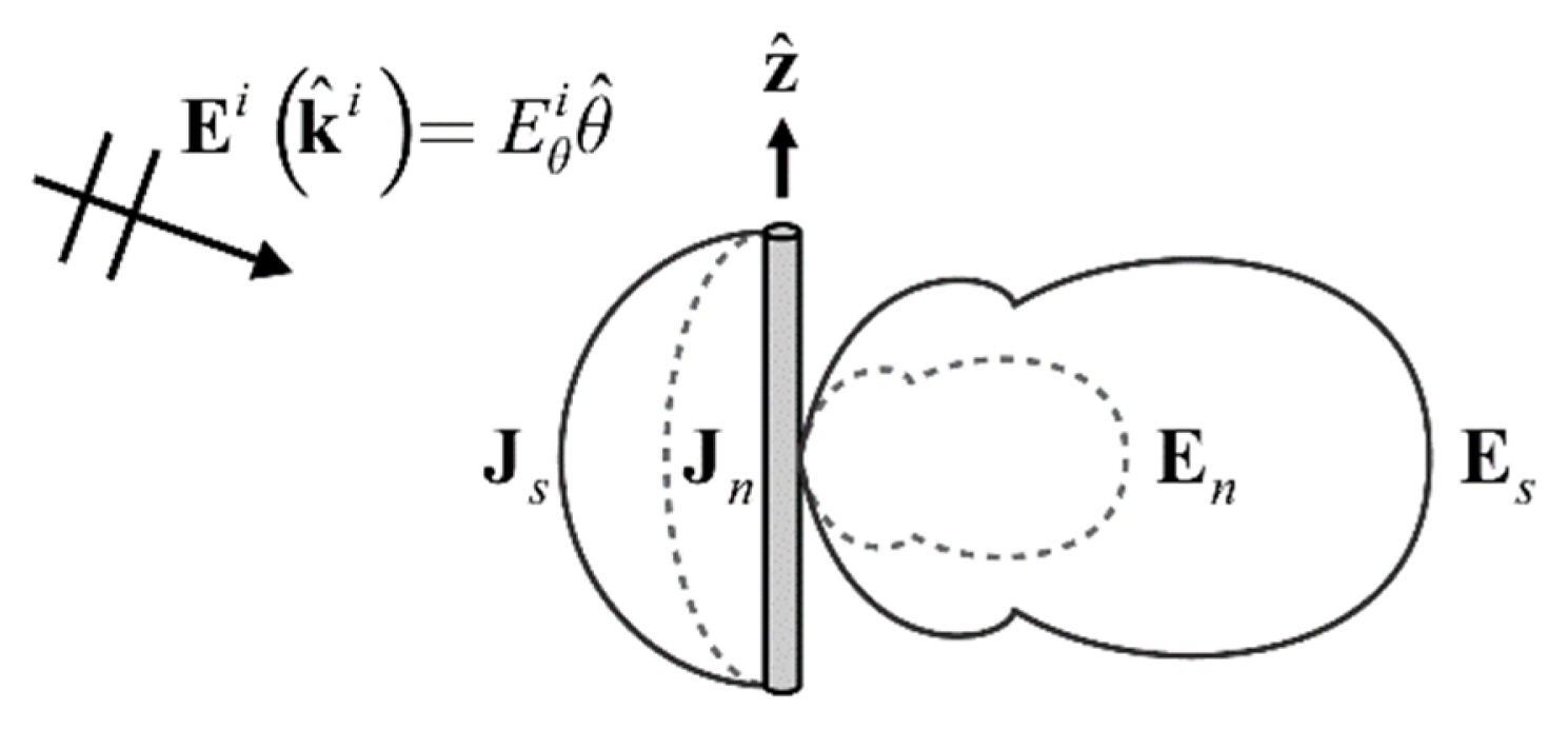
In this work, a linear wire scatterer was chosen because of its simple current distribution and linear polarization. Let us suppose that a wire scatterer is aligned along the z-axis, as shown in Fig. 2, and a plane wave of unit amplitude with an arbitrary direction of propagation k╠éi is incident on the scatterer. Then, the current induced on the scatterer is dependent on only the ╬Ė component of the incident wave, and the shape of the current distribution should be essentially the same for a small scatterer. For a specific reference, current distribution, Jn, a plane wave incident in a direction k╠éi can be considered to induce the following current distribution:
where c(k̂i) is a function of the incident direction. If we can write the radiated field from the current distribution Jn as:
the scattered field due to wave incident in the k̂i direction can be written as:
where G(r) is the free-space GreenŌĆÖs function.
The equation indicates that the scattered field has the same pattern, except for the amplitude, regardless of the direction of the incident wave. Since the compensation method is derived from these characteristics, the wire scatterer needs to be electrically small. If the other scatterer geometries are considered, they must meet the conditions above.
The scattering (re-radiation) pattern of the wire scatterer, having a wide beamwidth, linear polarization, and smooth shape without a side lobe, could be advantageous for scatterer compensation and phase restoration.
1. Scatterer Compensation
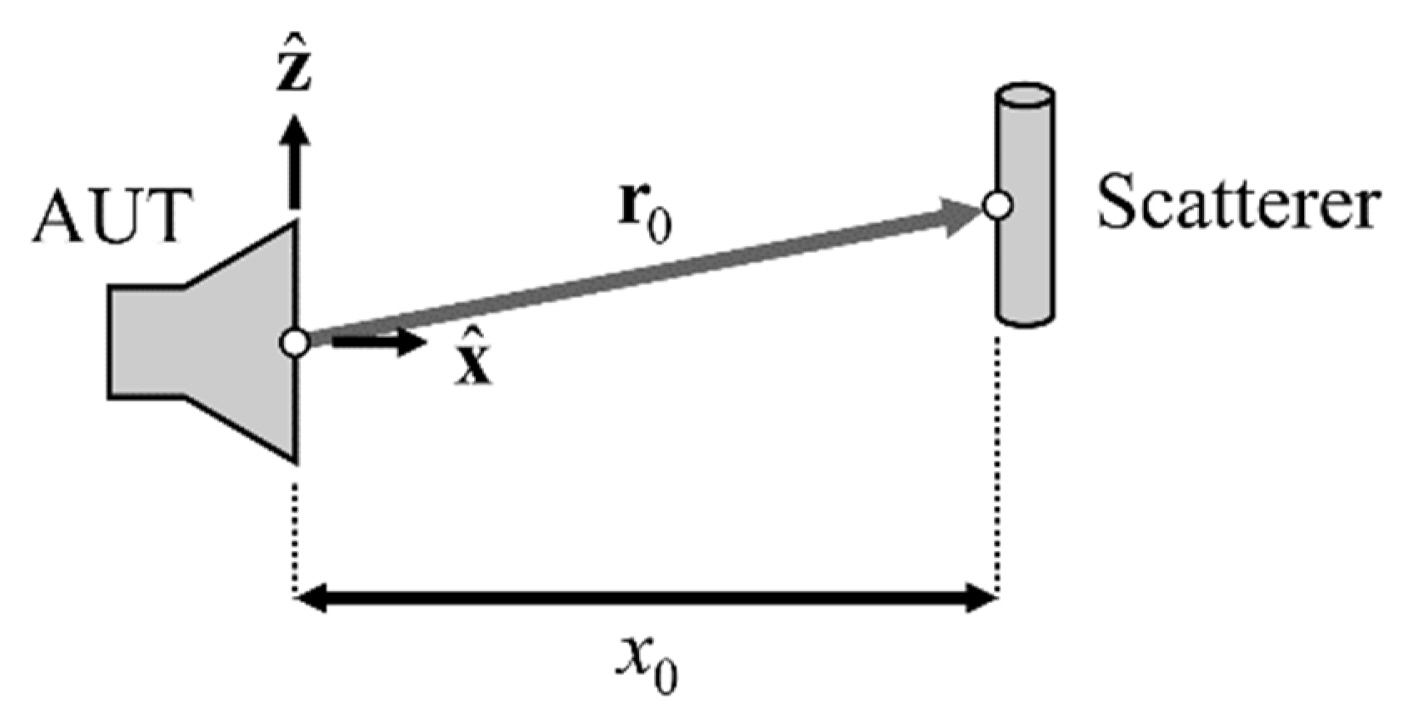
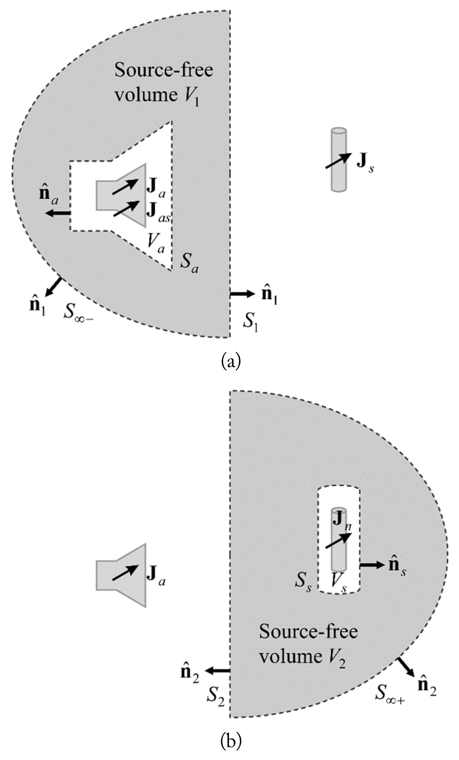
Fig. 3 shows the geometry of an AUT and a scatterer in isotropic and lossless media. The AUT at the coordinate origin is connected to a port, which is both transmitting and receiving, and the scatterer is in the plane x = x0. Suppose that the current on the AUT is Ja, which is produced by the source generator. When there is no scatterer, Ja produces the fields Ea and Ha. When the scatterer is present, Js is induced on the scatterer due to Ea and Ha. Then Js is reradiated to produce Es and Hs, and subsequently Jas is induced on the AUT due to Es and Hs. These are shown in Fig. 4(a). Higher-order interactions are ignored for simplicity of explanation.
In the simplified geometry described above, there are two states. Ja, Ea, and Ha are present for a state when there is no scatterer, and Ja + Js + Jas, Ea + Es + Eas, and Ha + Hs + Has are present for the other state when there is a scatterer.
First, we show that what we measure on the scanning surface S1 is electromagnetic power coupled between the AUT and the scatterer by applying the reciprocity theorem between the two states in the two regions. For the AUT volume Va, which is enclosed by the closed surface Sa, the reciprocity applied for the two states can be described as [1, 10]:
The products Ea ┬Ę Jas, Eas ┬Ę Ja, Ea ├Ś Has, and Eas ├Ś Ha vanish due to the symmetry, and the induced current on the scatterer Js does not exist in Va [11]. Therefore, (10) can be simplified as:
where r0 is the position vector between the AUT and the scatterer. It can be thought that Pa(r0) is proportional to the open-circuit voltage produced by the scattered field of the scatterer and could also be related to the S-parameter as follows:
Next, we consider the reciprocity theorem between the two states for the source-free volume V1, which is enclosed by S1, SŌł×ŌłÆ, and Sa. In this source-free region, the reciprocity for V1 can be written as:
Because all fields should be plane waves at SŌł×ŌłÆ, the integral Ōł½SŌł×ŌłÆ { } ┬Ę n╠é1 da = 0. We then obtain the following:
where n╠é1 = ŌłÆn╠éa. By applying the reciprocity theorem in the two regions, we obtained the same quantity Pa(r0). Thus, the electromagnetic power coupled between the AUT and the scatterer passing through S1 can be measured using Pa(r0) at AUT.
Now, consider the geometry in Fig. 4(b), which shows the volume containing the scatterer. Suppose that we can model the scatterer as a wire antenna with a pair of imaginary terminals. An independent current source with In is placed across the terminals, producing the current Jn on the scatterer, which then produces En and Hn. Applying the reciprocity theorem in volume Vs and in the source-free volume V2, we can obtain the following two equations for the two volumes:
and
where the higher-order interactions are ignored. If the scatterer is electrically small, we can define In such that
where Voc is the open-circuit voltage across the terminals of the scatter due to fields Ea and Ha. From (15), (16), and (17), we can obtain the following:
Note that the current induced on the scatter due to the fields Ea and Ha is a scaled version of Jn, as shown in (7). In elaborating (17), Ea and Ha can be thought to induce an open-circuit voltage Voc across the scatterer terminals. The current across the terminals of the scatterer could be Voc/Zs, where Zs is the input impedance of the scatterer. Thus, (7) can be rewritten as:
If we take that the surfaces S1 and S2 are identical, and n╠é1 = ŌłÆn╠é2 in (21), using (12) we can obtain the following:
where ╬▓ is a proportionality constant.
Eq. (22) represents the relationship between the fields produced by Ja and Jn in the near zone. The above relationship can be transformed into a new relationship in the far field by using the plane wave spectrum and Fourier transform [11]. Here, we adopted the process described in [11] and [12]. Fields in the far zone can be represented using a spherical coordinate system (r, ╬Ė, Žå), and the related wavenumber can be expressed as k = ksin╬Ė cosŽåŌŚ»+ksin╬Ė sinŽå ┼Ę+ k cos╬Ė z╠é. When the near-field plane S1 is the yz-plane located at x = x0, (22) can be written as:
(23)
where
E a ŌĆē ( ╬Ė , Žå ) = E ╬Ė a ╬Ė ^ + E Žå a Žå ^ E n ŌĆē ( ╬Ė , Žå ) = E ╬Ė n ╬Ė ^ + E Žå n Žå ^
(24)
and
(25)
where
and
IV. Experiment and Validation
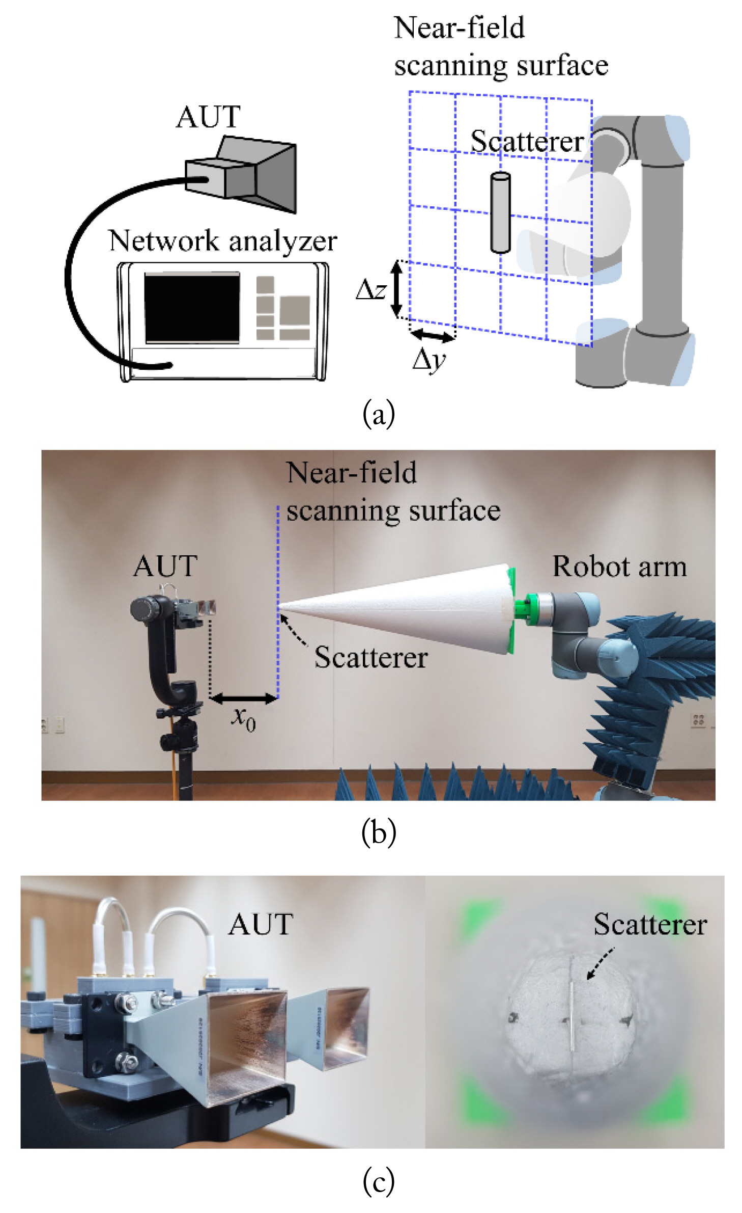
To verify the performance of the one-port near-field antenna measurement technique with a small wire scatterer, we performed a radiation pattern measurement. Fig. 5 shows the measurement setup. A 2 ├Ś 1 horn antenna was used as an AUT because it has significantly different near-and far-field patterns. A 0.68 cm long wire with a diameter of 0.5 mm was used as a scatterer. The length of the wire was chosen to be a half wavelength at the highest frequency of interest. A robot arm scans the scatterer over the near-field scanning surface, whereas a network analyzer measures the S11 at frequencies from 15 to 22 GHz at each grid point. The scanning surface was 5 cm from the AUT and 20 cm ├Ś 20 cm in area with a 0.2 cm grid spacing. The measurement area was empirically chosen such that the variation over the main lobe is relatively small. The spacing needs to be less than a quarter wavelength according to the Nyquist theorem, which is 0.34 cm. In practice, slightly less spacing interval is desired, and we chose 0.2 cm for simplicity. To reduce the reflections from the robot arm, the scatterer is located at the top of a 50 cm high truncated expanded polystyrene (EPS) cone, whose bottom is attached to the robot arm.
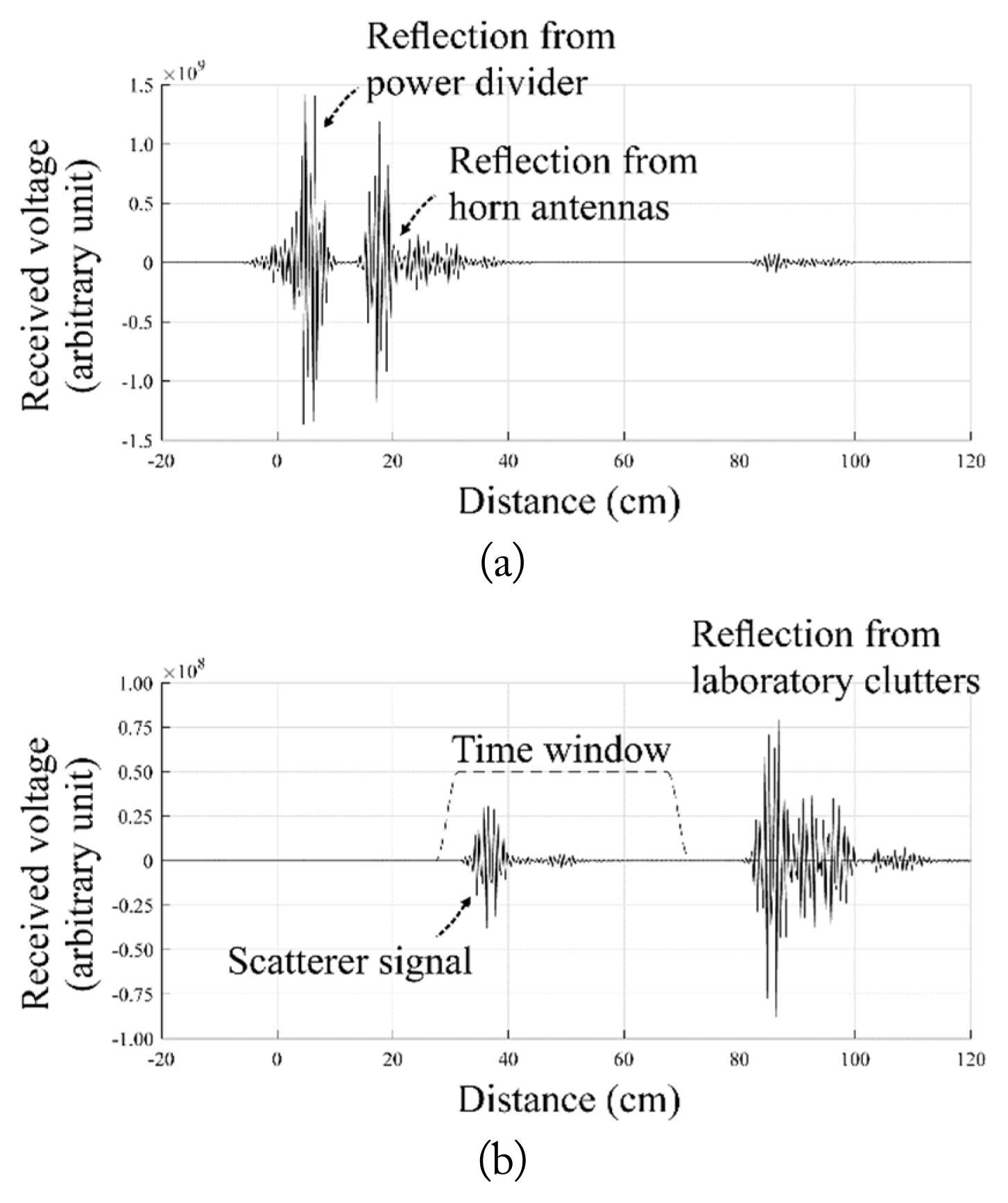
In many cases, the AUT may not be matched to the driving circuit. Therefore, the reflections from the input port could be significant. The AUT consists of two horn antennas, cables, and a power divider. The time-domain waveform shows the internal reflections from these components, as shown in Fig. 6(a). To remove these internal reflections, we measure the differences between the signal with the scatterer, S11, and the signal without the scatterer, S11ŌĆ▓. Because both S11 and S11ŌĆ▓ contain the same internal reflections, we can obtain the signal without the internal reflections from ╬öS11 = S11ŌĆōS11ŌĆ▓. The time-domain waveform of ╬öS11v for r0 = (x0, 0, 0) is shown in Fig. 6(b). To further reduce the signals from laboratory clutter, such as the robot arm, walls, and floors, time gating was applied.
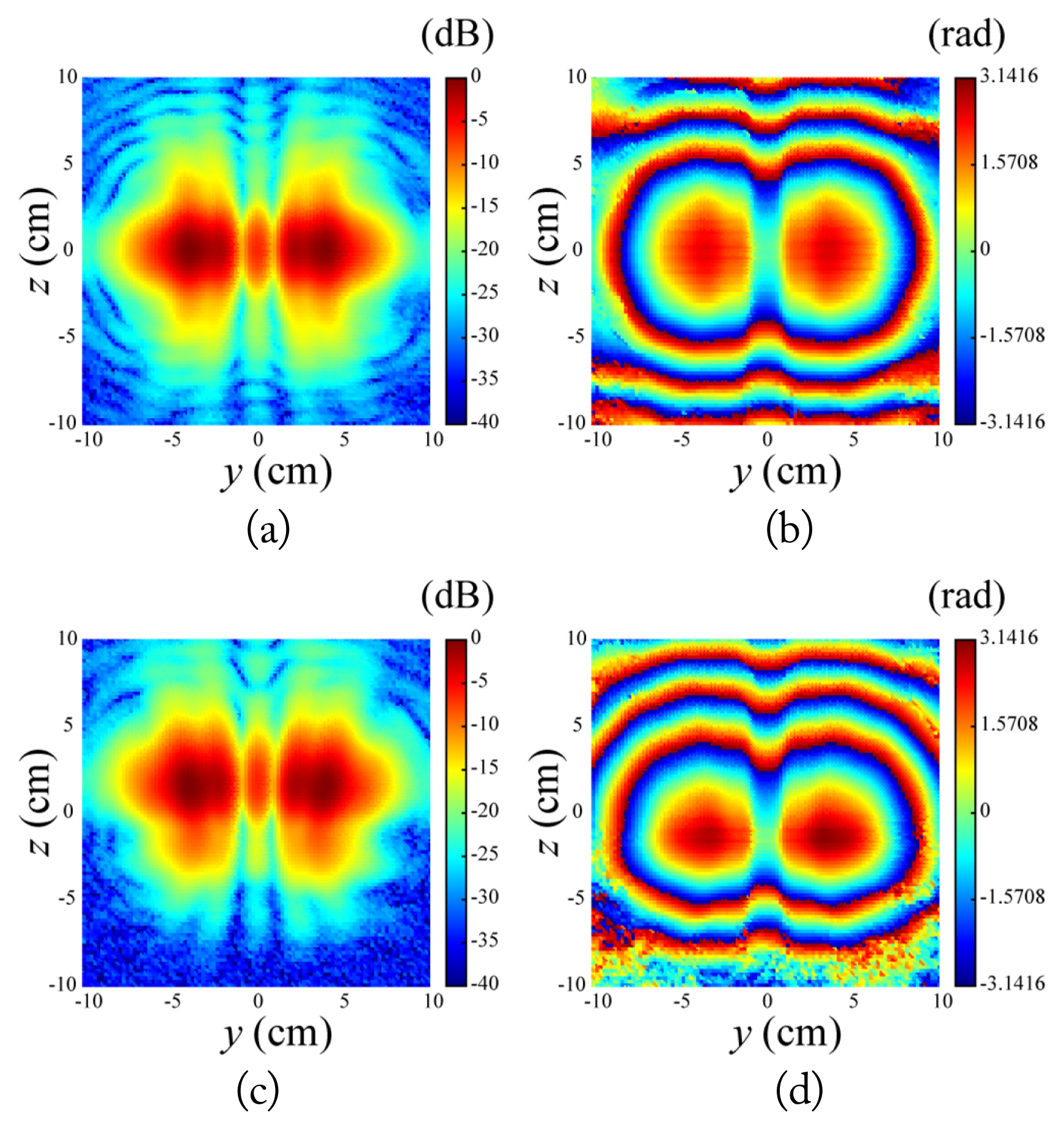
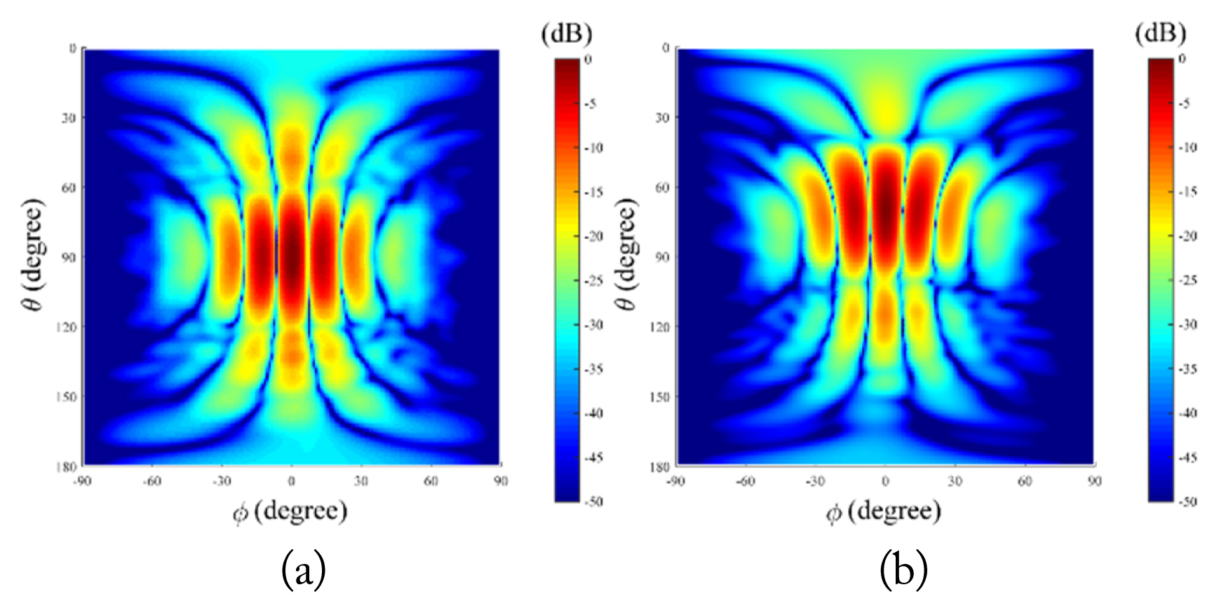
Fig. 7 shows the measured amplitudes and phases of the near-field data from the vertically aligned scatterer at 18 GHz. Fig. 8 shows the far-field radiation patterns obtained from the proposed compensation method at 18 GHz. The phases were restored using the weighted least-squares 2D phase unwrapping method [9]. Figs. 7(a), 7(b), and 8(a) were obtained by having the main beam of the AUT aligned to the x-axis, and Figs. 7(c), 7(d), and 8(b) were obtained by tilting the main beam by 20┬░ in the E-plane. The figures show the near-and far-field pattern differences and the well-transformed radiation patterns with the main beam in the corresponding tilt angles.
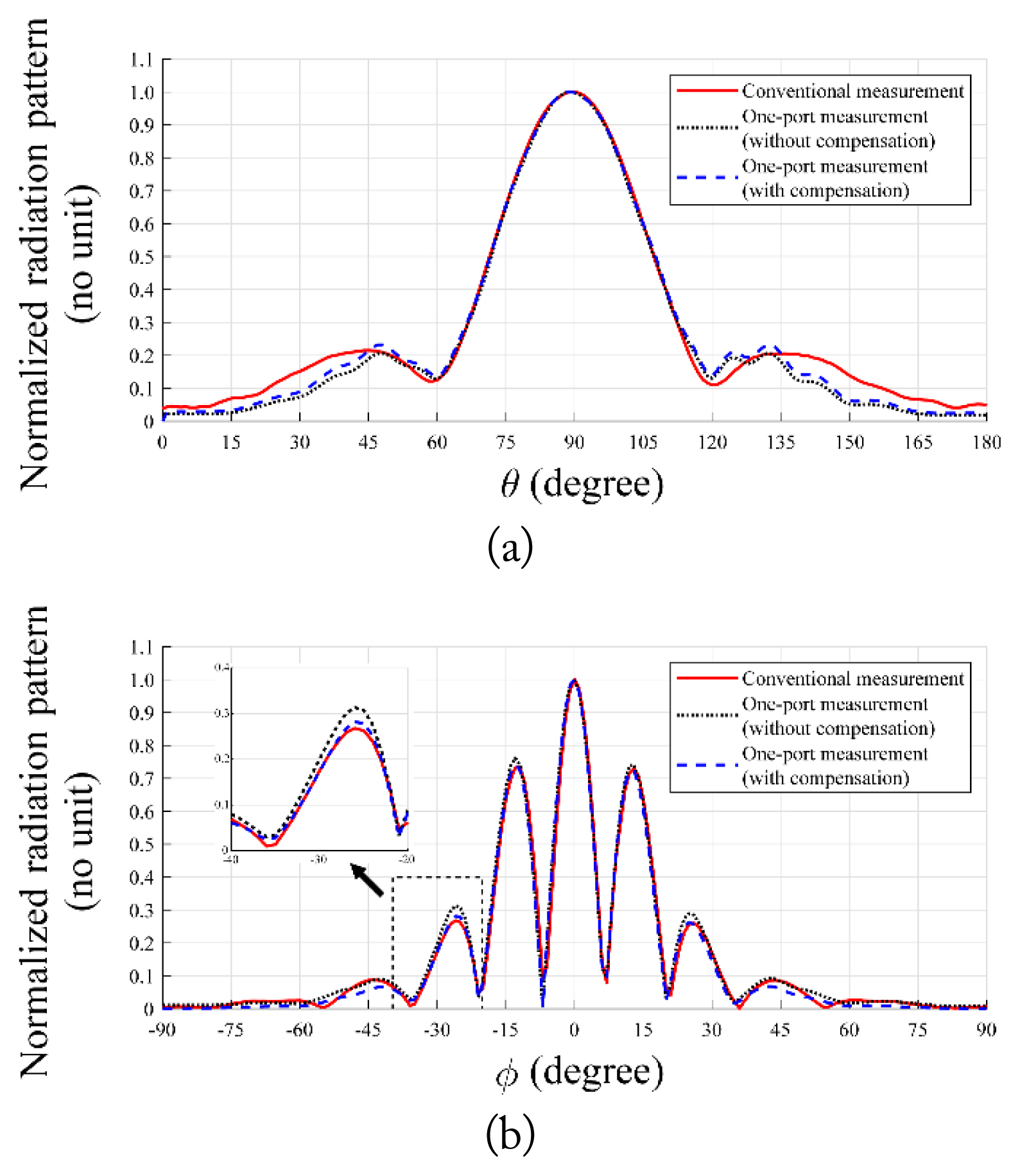
In order to show the accuracy of the proposed method, the radiation patterns obtained from the proposed method are compared with those measured in a conventional direct measurement facility, which is a 16 m ├Ś 11 m ├Ś 9.5 m commercial anechoic chamber. Fig. 9 shows the radiation patterns of the AUT in both the E-and H-planes at 18 GHz. The red solid lines show the conventional measurement, and the blue dashed lines and black dotted lines show the proposed measurement with and without the proposed compensation, respectively. As shown in the figures, the proposed measurements, both with and without the proposed compensation, agree well with the conventional measurement within the range of ┬▒30┬░ from the center. Because the planar scanning surface is suitable for the directive antennas, only the patterns near the center are considered accurate. Nevertheless, the compensation method still shows the improvement in the off-center region, so the agreement is closer to the proposed compensation.
Thus, the proposed one-port near-field antenna measurement technique was validated for a planar scanning surface.
V. Conclusion
In this work, a one-port near-field antenna measurement technique with a small wire scatterer was proposed. In the conventional near-field measurement technique, a probe antenna is scanned in the near-field scanning surface with a sampling interval of less than a half wavelength. The S21 parameter was measured between the probe and AUT. The data obtained in the near-field were transformed to the far-field pattern. The probe radiation pattern was compensated for better measurements. However, in the proposed technique, a wire scatterer is scanned with an interval of less than a quarter wavelength, and the measurement is made only at the port of the AUT. The 180┬░ phase uncertainty was removed by applying a 2D phase unwrapping method. The data obtained in the near-field were transformed to a far-field pattern. The scatterer scattering pattern was compensated for better measurements.
The proposed measurement technique was validated by measuring the radiation pattern of an AUT, which is a 2 ├Ś 1 horn antenna. The far-field radiation pattern obtained using the proposed technique was compared with that obtained from a conventional commercial anechoic chamber. It was shown that they agree well, especially in the region near the center, which is expected because of the nature of the rectangular near-field scanning surface. In future studies, the precision of the proposed technique will be further improved by enhancing the scattered signal using other types of scatterers.