Efficient Recurrent Neural Network for Classifying Target and Clutter: Feasibility Simulation of Its Real-Time Clutter Filter for a Weapon Location Radar

Article information

Abstract

I. Introduction

Recently, artificial intelligence (AI) technology has been successfully incorporated in a wide range of applications with emphasis on image and language processing. Due to the rapid development of computer technology, deep learning (DL) in an artificial neural network (ANN) has succeeded by using a massive dataset [1, 2]; this has drastically improved the ANN’s precision. Many ANN structures, such as the convolutional neural network (CNN), recurrent neural network (RNN), and deep belief network (DBN), have been proposed, each having its advantages and disadvantages. A CNN can show performance comparable to that of an RNN for sequential data processing but has a higher computational load [3]. Therefore, RNN networks have been commonly applied to sequential data training in language recognition and time-series analysis [4, 5].

In the radar industry, machine learning (ML) or DL techniques have been used in diverse areas such as synthetic aperture radar (SAR) applications [6, 7], jamming detection and classification [8], target detection and recognition [9–11], clutter suppression [12], and radar resource management [13]. In this paper, an ML technique is used to classify the artillery projectiles and radar clutter that are tracked by the weapon location radar (WLR) developed by LIG Nex1. This radar can simultaneously detect and track artillery projectiles fired by several guns. As a result, the radar data is sequentially measured in the time domain. For this kind of classification, an RNN can be used to increase the radar’s tracking capability when clutter tracking is terminated at the initial tracking process. It is important to reduce the probability of misclassifying the target as clutter. Also, the classifier design should be numerically efficient and provide a robust and highly reliable classification probability, even for an insufficient or highly imbalanced dataset, common in a radar measurement campaign. The WLR’s target classification is reported in [14]; it only considers targets without clutter data.

In Section II, the measured dataset and its preparation for RNN training are addressed. A feature dimension reduction scheme is proposed. Then, in Section III, the performance of the trained RNN is assessed, and a simple method of enhancing its accuracy is proposed. Finally, the feasibility of using the RNN classifier to perform real-time rejection of clutter is investigated.

II. Data Preparation

The WRL collected the dataset using two tracking filters, a simple Kalman filter (KF) and an extended Kalman filter (EKF). The filter designs were based on an interacting multiple model (IMM) that assumed constant velocity/acceleration of the measured objects. The EKF updated the target position in range and sine space angle (RUV coordinates): U = sin (Az) and V = sin (El). Here, Az and El are the azimuth and elevation angles in antenna coordinates where the antenna is in the xy-plane. The overall precision of the dataset collected by the EKF may be generally higher than that of the KF which can reduce the error caused by the nonlinearity of the coordinate transformation [15]. Four artillery projectiles were measured: gun heavy/light (GH/GL), mortar heavy/light (MH/ML), rocket heavy (RH), and rocket-assisted projectile (RAP). Table 1 shows the total number of targets and the clutter dataset. For the EKF datasets, only GH and MH have been measured so far.

Table 1

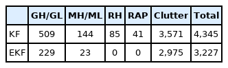
Number of measured datasets for four targets and clutter for the KF and EKF filters

Since the radar detected and tracked many clutters returns during the measurement, the clutter dataset is much larger than that of the other targets. The clutter is mainly categorized into two major object types: natural ones like clouds or birds and manmade ones like fixed- or rotary-wing aircraft. The raw measurement data consists of eight different data sets collected at discrete time points, t_n (in s) for n = 1 … k, among which three sets are used to train and test an ANN: target position ⇉(t_n) (in m), radial velocity v_r(t_n) (in m/s), and radar cross-section (RCS) (in m²) or signal-to-noise ratio (SNR). The position was measured in antenna coordinates and transformed based on the inertial navigation system to local east, north, up (ENU) Cartesian coordinates for the radar location.

1. Feature Selection and Transformation

Target tracking started when the target was detected and ended when sufficient tracking data was collected to extract ballistic parameters like the drag coefficient. During tracking, the data was updated at every sample time. When the radar temporarily lost the target track, it tried to detect the target at the next sample time and predict its position without an EK or EKF update (memory track). If the track was successfully restored, then the radar kept tracking the target. If not, the track was terminated after 1–5 trials [16]. This means that the data sequence length varies and can have missing values. Since the missing data may negatively affect the performance of the classifier, the data is linearly interpolated at the missing points [17]. All the initial times and positions of the data t_n – t₁ and ⇉(t_n) – ⇉(t₁) = (E, N, U) in ENU coordinates.

Targets usually fly in a specific direction, but true clutter tracks are typically random. Thus, their most distinguishing feature might be their position sequence. Fig. 1 shows 10 samples of the adjusted position of the MH shell and clutter collected by the KF. Most of the clutter tracks are random, but some are very similar to that of the target, for example, “a” in Fig. 1(b). Since MH shells fly at a lower altitude than other targets, the received signal is highly contaminated by ground clutter as can be seen in Fig. 1(a). The RCSs of the artillery projectiles are very small, while that of the clutter is widely distributed as seen in Fig. 2. Thus, RCS may not be a suitable feature for this classification problem. Also, radial velocity does not clearly distinguish targets from clutter.

Fig. 1

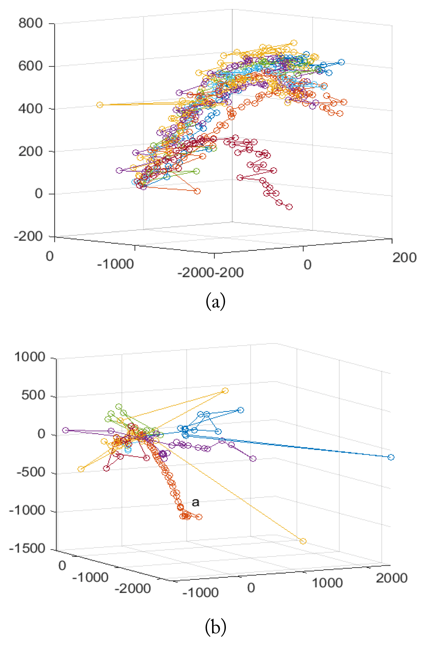
Measured position samples of KF dataset in ENU coordinates: (a) MH and (b) clutter.

Fig. 2

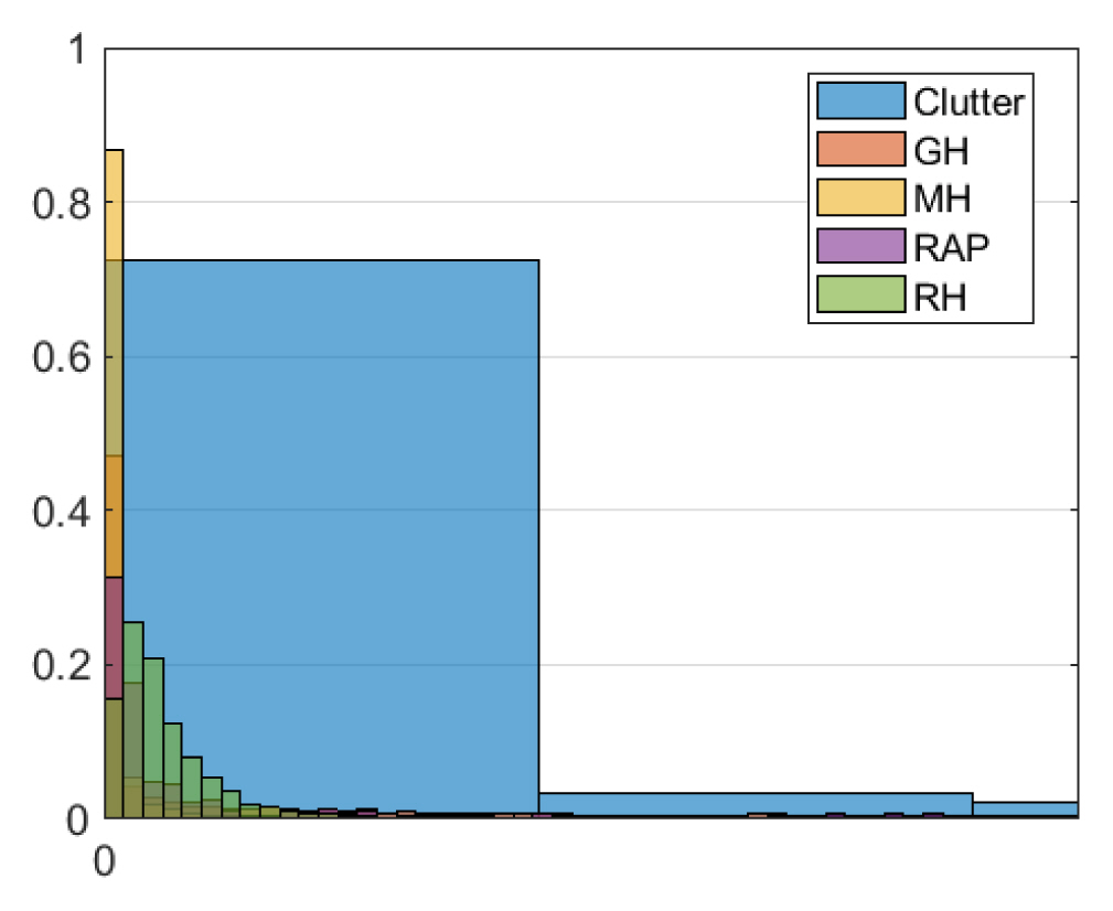
Probability density function of RCS collected by KF for four targets and clutter.

To maximally separate artillery projectile returns from clutter, positions were converted into three more features called Case 1, 2, 3, and 4. Case 1 is the measured position, (E, N, U). Case 2 is the position difference as in Δ⇉(t_n) = ⇉(t_n+1) – ⇉(t_n). To reduce the dimension of this feature, the normal vector to a plane containing ⇉ and –Û is considered. Since the normal vector is two-dimensional, the slope of a line orthogonal to the line from the origin to (E, U) may be a good alternative; it is one-dimensional and is simply calculated by –E/N. This is called Case 3. For Case 4, a similar slope is computed based on the differences as in –ΔE(t_n)/ΔN(t_n). Fig. 3 shows the probability density function (pdf ) of four KF positions where the y-coordinate is plotted for Cases 1 and 2. Fig. 4 shows the identical pdfs for the EKF positions. In Figs. 3 and 4, for clear comparisons, the means of Case 2 and 4 are added by 2000 and 10, respectively. Similarly, the means of Case 2 and 4 are larger by 3000 and 10, respectively. For the training/test datasets, the position, radial velocity, and RCS were selected. Hence, the dimension of the input features is five for Cases 1 and 2; four for Cases 3 and 4. Of the whole dataset, 70% was randomly selected for training and 30% for tests.

Fig. 3

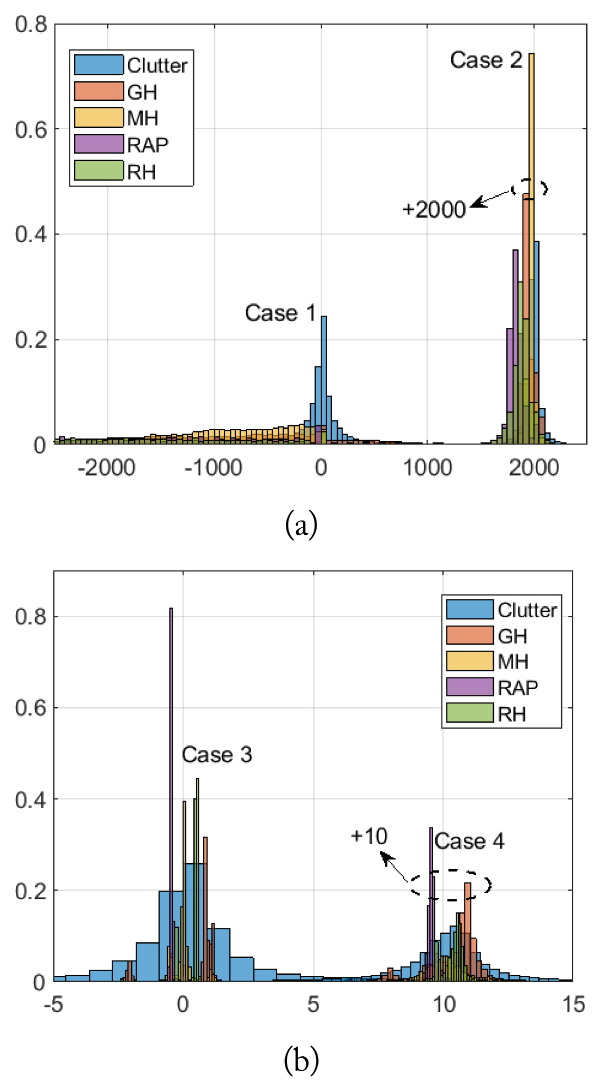
Probability density function of positions collected by the KF: (a) the y-coordinate for Cases 1 and 2 and (b) the slope for Cases 3 and 4.

Fig. 4

Probability density function of positions collected by the EKF: (a) the y-coordinate for Cases 1 and 2 and (b) the slope for Cases 3 and 4.

III. Training Network and Performance Assessment

Binary and multiclass classifiers were trained by the weighted cross-entropy loss method to partially compensate for the imbalance of the dataset as seen in Table 1 [18]. The weight was simply calculated by the ratio of the size of target and clutter data to the total data size. The binary classifier sorts objects into two categories as “target” and “clutter,” while the multiclass classifier produces five categories of four types of artillery projectiles and clutter.

The ANN consists of two long short-term memory (LSTM) layers as regression and classification layers. The regression layer receives the input sequence, and the classification layer outputs a final classification label. The number of hidden cells for the first and second layers are denoted as N₁ and N₂, respectively. To prevent the ANN from overfitting, a dropout layer is inserted between the two LSTM layers, and the dropout factor is assumed to be 0.1. The RNN is trained over 100 epochs. For fast training, the data is divided into a batch of data whose size is fixed at 50. At each epoch, the training data is randomly shuffled. First, the RNN is trained by the KF dataset since it is larger than the EKF dataset. Table 2 shows the accuracy of the binary RNN classifier for several values of N₁ and N₂. Four different networks can be trained as classifier k using the Case k dataset for k = 1, 2, 3, and 4.

Table 2

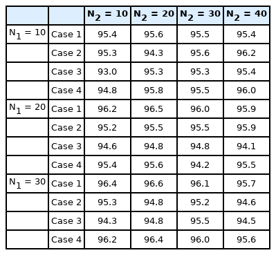
Accuracy (%) of the binary classifier trained by the KF dataset

Table 3 shows the accuracy of the multiclass classifier. Due to the reduction of one feature dimension, the accuracy of classifier 3(4) is slightly less than that of classifier 1(2), but it can be seen that accuracy for all classifiers is almost constant for two classifications.

Table 3

Accuracy (%) of the multiclass classifier trained by the KF dataset

Table 4 shows the accuracy of the two classifiers trained by the EKF dataset for a fixed N₁ = N₂ = 20. Although the number of datasets and the types of artillery projectiles are smaller than those for the KF dataset, the accuracy is improved. The multiclass classification probabilities are lower than those in [14] because the effect of clutter is much larger, but the EKF results are comparable to those in [14]. Based on Tables 2–4, it can be seen that 20 hidden cells for two layers may be sufficient. For the rest of the simulations, therefore, 20 cells were assumed for two LSTM layers and the binary classifier was further investigated.

Table 4

Accuracy (%) of classifiers trained by the EKF dataset

To increase the size of the test data, the training and test datasets were combined into one test dataset. Table 5 shows the accuracy of two binary classifiers. Since 100 epochs are not sufficient for complete training, the overall accuracy of the classifiers in Table 4 degenerated as shown in Table 5, especially for the KF. The accuracy of an RNN classifier, however, is always higher than that of the best conventional tree algorithms such as the bagging tree algorithm.

Table 5

Accuracy (%) of the binary classifier for the combined dataset

When the dataset is sufficient, a single classifier trained by all input features may produce a good performance, but in this paper, the size of the dataset is not large. More hidden cells are required to increase the accuracy of the classifier which is not numerically efficient. Since the input features for each dataset case can capture a different physical mechanism of the track as seen in Figs. 3 and 4, a simple combination of two classifiers can significantly decrease misclassification probability. For example, classifier 1 and 3 could be used as a primary and a secondary classifier, respectively. If the two classifiers predict the same label, it becomes the final label of the combined classifier. If not, the label produced by the primary classifier flips to the other label. Fig. 5 shows the block diagram of the combined classifier; it can be extended to a real-time classifier with a given threshold probability. The number of erroneous predictions is summarized in Tables 6 and 7 for two datasets. For this simulation, the threshold is assumed as 1.

Fig. 5

The block diagram of combined classifier with threshold.

Table 6

Number of classifier labeling errors for the KF dataset

Table 7

Number of classifiers labeling errors for the EKF dataset

The diagonal numbers in Tables 6 and 7 are the result of a sole classifier, while the off-diagonal numbers are those for the combined classifier. For example, 181 (5.1%) at the second row and third column in Table 6 is the mislabel number (probability) if classifier 1 and classifier 2 are used as the primary and secondary classifiers, respectively. The combination of classifier 2 with 3 or 4 can provide the highest accuracy. For example, the combination of classifier 2 and 3 can reduce the misclassification probability from 3.6% to 1.0% and 18.4% to 2.7% for “target as clutter” and “clutter as target” labels, respectively, compared with those of the sole classifier 2 for the KF dataset. Table 7 shows a similar reduction of mislabeling probability for the EKF dataset. Hence, a combination of classifier 2 with 3 or with 4 may be appropriate for both the KF and EKF datasets. Fig. 6 shows the target and clutter tracks mislabeled as clutter and target by the combined classifier 1(3) and 4 for the EKF dataset. The mislabeled target and clutter tracks are similar to those in Fig. 1(b) and 1(a), respectively.

Fig. 6

The misclassified tracks for the EKF dataset in ENU coordinates: (a) target using classifier 3 and 4, (b) clutter using classifier 1 and 4.

Since the trained RNN is swallow, its real-time computation may be feasible. To estimate the real-time performance of the classifier, the features were sequentially inputted to the network. If the predicted probability of one of two labels was greater than a given threshold, then the network would output the classification label. Table 8 shows the overall accuracy of the real-time simulation of the four trained classifiers for two threshold probabilities, 80% and 90%. The mean ratio of the required length of the sequence to the total length for termination is also summarized. About 50% of the sequence is required for termination. Tables 9 and 10 show the misclassification number (probability) for the proposed combined classifier for the KF and EKF datasets, respectively. The combination of classifiers can drastically improve the final accuracy.

Table 8

Accuracy (%) of the real-time classifier and mean ratio of the required length to the total length of the sequence for termination

Table 9

Number of mislabels for real-time classifiers for the KF set

Table 10

Number of mislabels for real-time classifiers for the EKF set

Similar to the previous analysis, the combined classifiers 2 with 3 and 1 with 3 may be the best for the KF and EKF datasets, respectively. After a 58% tracking process, the mislabel probability for “target as clutter” was reduced from 4.5% to 1.6% for the KF dataset and from 4.5% to 2.4% for the EKF dataset with the 90% threshold probability, respectively.

The computer used to train the proposed network comprised an Intel Core i7-4930K CPU running at 3.40 GHz with 64 GB of RAM. The training time was within 5–10 minutes.

IV. Conclusion

To classify artillery projectiles and clutter tracked by a weapon location radar, an RNN classifier was trained with a real measured dataset. The data was collected by the radar using two tracking filters, a KF and an EKF. The sizes of the KF and EKF datasets are 4,345 and 3,227, respectively, and are highly imbalanced. The dataset clutter portion is around 82% and 92% for the KF and EKF, respectively. KF data for four types of artillery projectiles and EKF data for two of those types were collected. To clarify the radar signature difference between the artillery projectiles and clutter, the input data were selected and converted to four different input feature expressions. Then, binary and multiclass RNN classifiers were trained with the weighted cross-entropy loss method to compensate for the class imbalance. It was shown that the performance of the classifiers is insensitive to the number of hidden cells. Thus, 20 hidden cells were assumed for two layers for further analysis. The multiclass classifier’s accuracy is less than that of the binary case, especially for the KF data. To increase the accuracy of the binary classifier, two classifiers were combined. When classifiers 2 and 3 are combined against the KF dataset, false probabilities decrease from 3.6% to 1.0% and from 18.4% to 2.7% for the mislabeling of ““target as clutter” and “clutter as target,” respectively. A similar reduction can be observed for the EKF dataset. For real-time applications, the trained RNN can be terminated when the predicted probability of one of two labels is greater than a given threshold. Below about 60% of the tracking process, usually 50%, the network can terminate. It is recommended that classifier 3 be combined with classifier 2 for the KF dataset and with classifier 1 for the EKF dataset. For these combinations, the mislabel of “target as clutter” probability is around 1.6% and 2.4% for the KF and EKF datasets, respectively. When more EKF target data is available, the final accuracy can be improved.

Article information Continued

References

Biography
Il-Suek Koh received B.S. and M.S. degrees in electronic engineering from Yonsei University, Seoul, Korea in 1992 and 1994, respectively, and he obtained his Ph.D. degree from the University of Michigan, Ann Arbor, MI, USA in 2002. In 1994, he joined LG Electronics Ltd., Seoul, as a Research Engineer. Currently, he is a professor at Inha University, Incheon, Korea. His research interests include numerical and analytical methods for electromagnetic fields and radar applications.
Hyun Kim received B.S., M.S., and Ph.D. degrees in electrical and electronics engineering from Yonsei University, Seoul, Korea, in 2002, 2005, and 2011, respectively. He is currently a research engineer in LIG Nex1, Korea. His main interests are in the area of numerical analysis, phased array antenna, and radar systems.
Sang-Hyun Chun received B.S., M.S., and Ph.D. degrees in microwave engineering from Kwangwoon University, Seoul, Korea, in 2005, 2007, and 2011, respectively. He is currently a research engineer in LIG Nex1, Korea. His main interests are in the area of transmit/receive modules and radar systems.
Min-Kil Chong received B.S. and M.S. degrees in electronics engineering from Geyongsang National University, Korea, in 1994 and 1996, respectively. He is currently a research engineer in LIG Nex1, Korea. His main interests are in the area of transmit-receive module, active phased array antenna, and radar systems.