


I. Introduction
The modelling and simulation (M&S) technique could be crucial in the radar research to save experimental costs for the performance assessment of a radar system [1]. Among radar systems, recently, an automotive radar has received attention because the global autonomous commercial vehicle market is rapidly growing. The test of the automotive radar requires considerable funds and resources, and so the M&S method is more beneficial, safer, and cheaper than real experiments [2, 3]. Commercial software (SW) is available for this kind of simulation [4ŌĆō6], but due to the complexity of the problem, a relatively simple technique, such as geometrical optics (GO), is used to calculate the radar echo signal from adjacent objects around the radar.
Given that GO is prone to limit the SWŌĆÖs accuracy, it is required to deploy more accurate and flexible technique to compute the radar echo signal from diversely shaped objects, such as cars, buildings, trees, humans, and potholes. For the more flexible applications, the physical optics (PO) scheme is available. Because it is based on the surface current of the objects, the object shape can be considered in a simpler fashion than the GO scheme. The iterative PO scheme is proved to be accurate, yet it entails a time-consuming computation [7]. To estimate the time-domain echo signal from dynamic targets, the RF specifications of the vehicle radar should be considered in detail, including frequency, polarization, chirp rate, bandwidth, and radar operations, such as frequency-modulated continuous wave (FMCW) radar. FMCW radar is prevalent among automotive industries [8, 9]. To calculate the backscattering by targets, the target geometry, material, and dynamics should be considered; however, most simulations have partially modeled the target with a small number of meshes or assumed the scattering centers of the target to create the time-domain echo signal because it is a substantially time-consuming job to fully account for the complete target geometry [10ŌĆō12]. Because the operating frequency of the vehicle radar is very high, the mesh number for the discretization of the target is very large, which limits the choice of the electromagnetic scattering calculation method [12, 13]. Recently, a numerical scheme has been proposed to compute the time-domain echo signal from a large target for an airborne radar system [7, 14]. The scheme adopts coherently integrated signals from the meshes inside an identical resolution bin. Because it ignores the interference effect among many meshes in the radar echo signal, we introduce a new method that can efficiently consider this interference effect.
In this paper, we propose an efficient numerical method to calculate the radar echo signal for a dynamic scenario based on the first-order PO scheme. This paper is organized as follows. In Section II, the proposed scheme to generate the time-domain echo signal is formulated. In Section III, the proposed scheme is verified, and a dynamic scenario is simulated, for which the performance of the proposed method is investigated based on the Range-Doppler (RD) map.
II. Signal Generation
1. Scenario and Generation of a 1D Time-Domain Signal
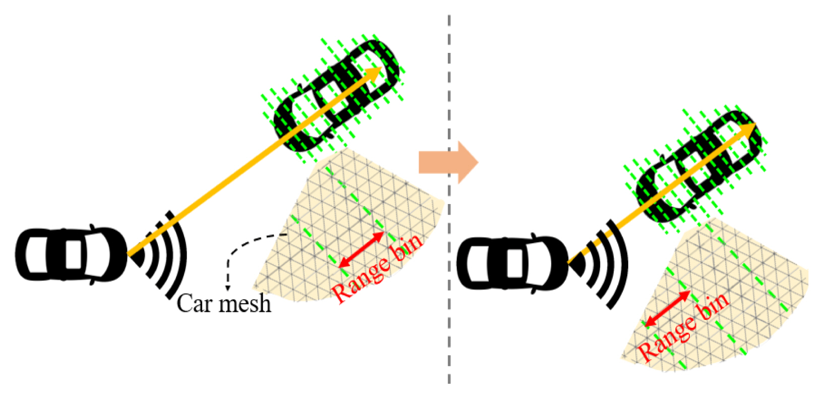
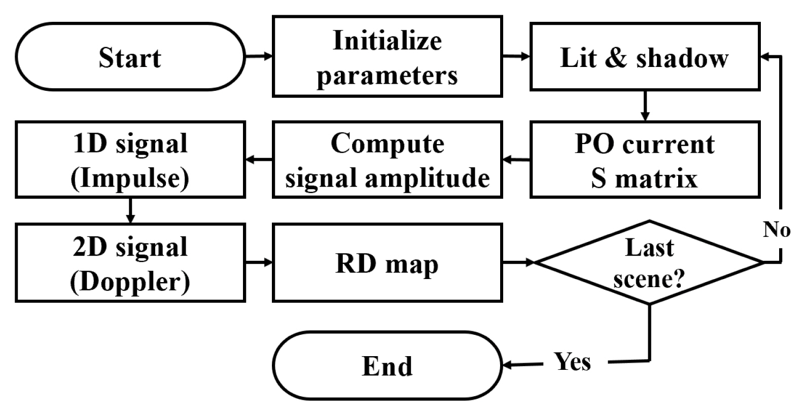
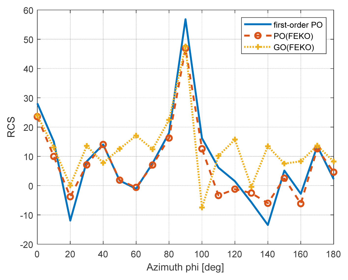
Fig. 1 illustrates the overall simulation scenario that considers the radar specification, target shape, and their dynamics. The position and velocity of the radar and targets are varied during the simulation. Triangle meshes on the target surface are also shown, which are grouped into several range bins. The bins are determined based on the relative positions of the radar and target. Fig. 2 presents a flow chart of the entire simulation process for a driving scenario. The radar echo signal is calculated at several time steps. At one time step, all objects are assumed to be in a stationary state until the next time step. The echo signal amplitude is calculated by the radar equation and the first-order PO scheme. The analytical formulation of the scattering matrix (S matrix) for an arbitrary triangle mesh is given in [15] for the PO scheme. The impulse response (1D signal) for a range bin consists of those from many meshes inside the range bin. Then, the 1D signal is repeatedly computed to form the 2D signal for the RD process. At the next time step, the radar and targets are relocated based on the given scenario, and the mentioned procedure is repeated until the final state of the scenario. To examine the accuracy of the first-order PO scheme, it is compared with the results of GO and PO schemes in the commercial tool, FEKO, in Fig. 3. The GO scheme adopts the full ray-tracing method, and the PO scheme considers up to the third reflection. The first-order PO scheme shows good agreement with two results.
To set up the driving simulation, configuration data are imported, including the target mesh and the simulator parameters, such as radar specifications and the dynamics of the radar and targets. The radar specifications consist of the carrier frequency, bandwidth, chirp duration time, transmission power, antenna gain, polarization, and its dynamics, such as the radarŌĆÖs initial position and the velocity vector. The radar is mounted on the car, whose beam is not oriented toward the ground. Hence, we can ignore the reflected signal from the ground. In all simulations, automotive models are assumed to be the Tesla S. The material is assumed to be a perfectly electrical conductor (PEC).
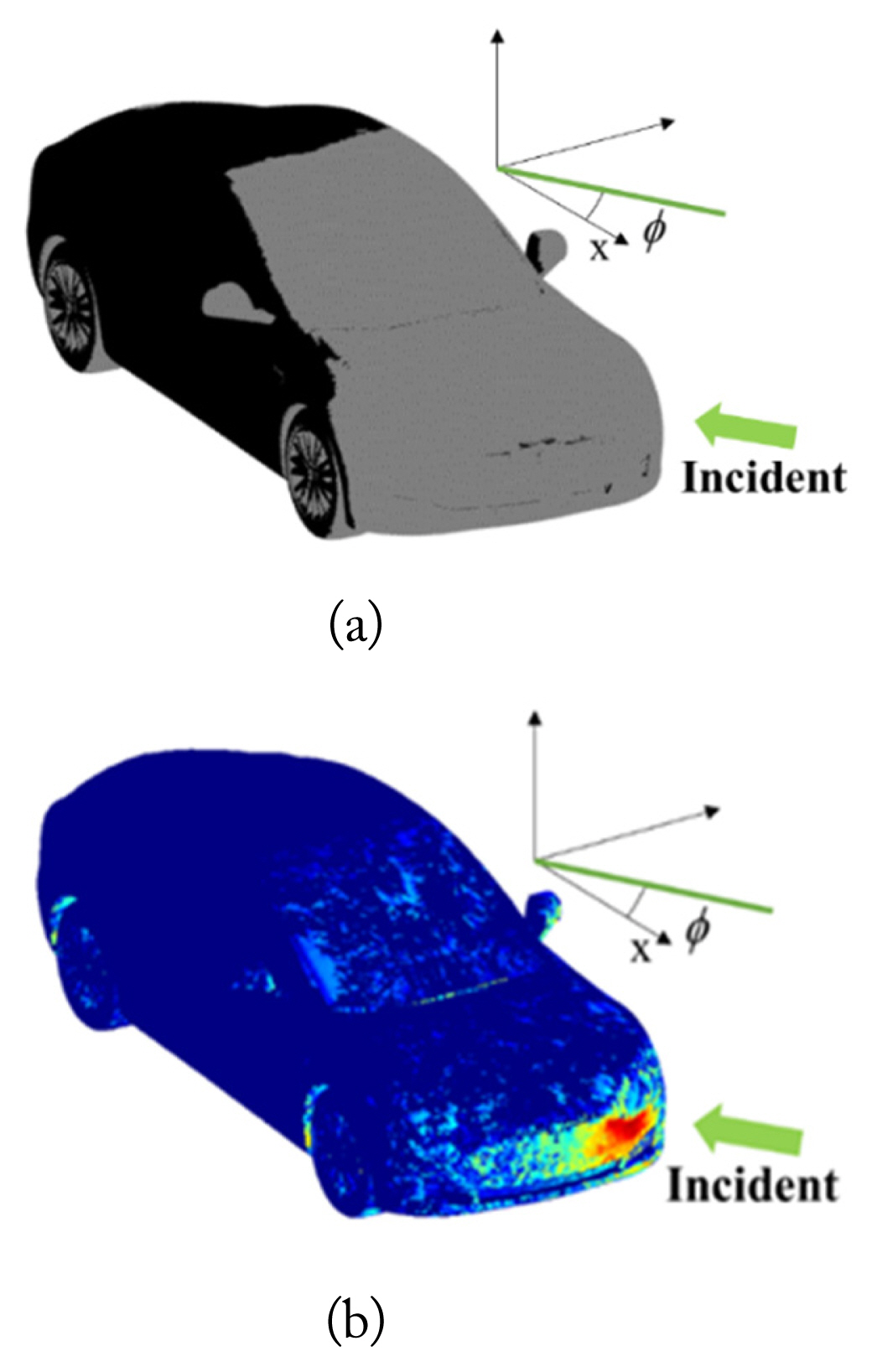
To calculate the echo signal from the targets at a chirp duration, first, the lit and shadow regions on the target surface are determined based on the incident angle of the radar signal on the target and the normal vector (n╠é) of each triangular facet. A complete determination of the shadow regions requires a very long computation time, but this simple method can generate a relatively accurate backscattering for a radar application [7]. Fig. 4(a) shows the lit and shadow regions, where lighter and darker colors are the lit and shadow regions, respectively, for a Žå = 20.63┬░ incidence. Around the tire and side mirror, the erroneous lit region is shown, but its backscattering contribution is small compared with that from the other lit region, as shown in Fig. 4(b). The S matrix for each mesh can be calculated by the first-order PO scheme, whose element is given by Spq, where p and q are the transmitted and received polarization, respectively. Then, the received power (Pr,k) from the kth mesh can be calculated by the radar equation as
where Pt is the transmitted power, Gr and Gt are the receiver and transmitter antenna gains, and ╬╗ is the wavelength. Rk is the range between the radar and the kth mesh. The radar antenna pattern is assumed to be a Gaussian pattern. The kth meshŌĆÖs radar cross section (RCS), Žāk, can be calculated by 4ŽĆ|Spq,k|2 [16]. Fig. 4(b) illustrates the RCS of each mesh in the dB scale, which clearly shows the hot spot for the incidence wave. Based on Eq. (1), the amplitude (Ak) of the echo signal from each mesh can be expressed considering the radar polarization as
where p╠é is the radar polarization unit vector, and ─źi and v╠éi are the h-pol and v-pol vector incidents on each mesh, respectively. ─źs and v╠és are the h-pol and v-pol vectors defined in the radar antenna coordinate, respectively. The FMCW signal is continuously transmitted to the targets, and then returned to the radar. Hence, the return signal is delayed in the time-domain due to the distance between the radar and mesh, and its amplitude can be estimated by Eq. (2). Its Doppler frequency shift is addressed in Section II-3. When the transmitted signal (st) is given by Eq. (3), the returned signal (sr) can be computed from the meshes as Eq. (4).
where fc is the carrier frequency, N is the number of meshes on the targets, and ╬▒ is the chirp rate. Žäk is the time delay of the return signal from the kth mesh given by 2Rk/c. Here, c is the speed of light. The returned signal is down-converted to the intermediate frequency (IF) band written as
where fIF is the intermediate frequency. Then, the range compressed signal (sExact) is obtained after Eq. (5) by going through the matched filter with the reference signal [9] as
where Žåk = i2ŽĆ (fIFt ŌĆō fcŽäk), T and BW are the chirp duration time and bandwidth, respectively. sinc(┬Ę) and ╬ø(┬Ę) are the sinc function and triangular function, t/T + 1 (ŌłÆT Ōēż t Ōēż 0) and ŌłÆt/T + 1 (0 Ōēż t Ōēż T), respectively. Because we consider the large structure and the high operating frequency, the Nyquist sampling rate (M) becomes very high. Hence, the numerical complexity becomes O(NM) to generate the returned signal from all meshes for one chirp signal, which is very time-consuming. Thus, to generate a complete 2D radar signal for a dynamic simulation, the direct computation of Eq. (6) is not efficient. An approximation scheme is required to reduce the complexity of Eq. (6).
2. Proposed Method
The echo signal Eq. (6) can be re-expressed with a reference signal (sRef) and impulses from each mesh as
where * is the convolution operator. sRef is given by
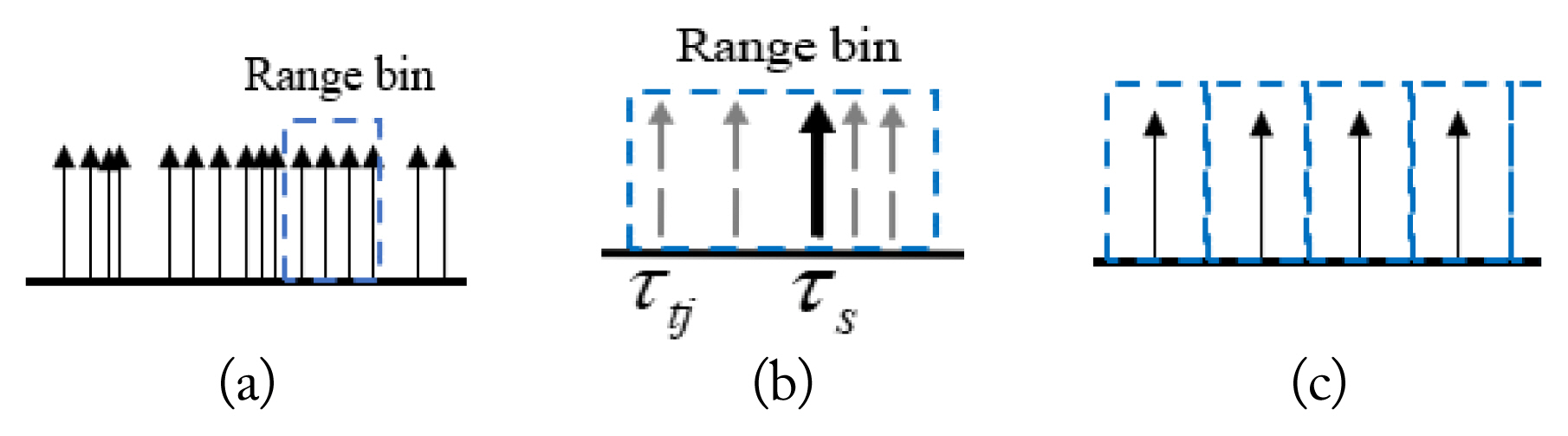
Fig. 5 shows an overall description of the proposed scheme to approximate Eq. (6). Fig. 5(a) illustrates the impulses from the meshes on the target. As seen in Fig. 1, one range bin can contain many meshes, which generate many impulses. The radar sample Eq. (6) or (7) at one sampling point (Žäs) inside a range bin as shown in Fig. 5(b) results in one impulse in each range bin shown in Fig. 5(c). Because the sampling point and the time locations of each impulse are different, as shown in Fig. 5(b), this should be compensated for. The time variable (t) in Eq. (8) is affected by the convolution process in Eq. (7). The exponential term (ei2ŽĆfIFt) in Eq. (8) is highly sensitive to the change of the time variable, but the variation of the product of the sinc and triangle function is small due to the small range bin size. Hence, a simple phase compensation may be sufficient, which can be given based on Eq. (5) by
Eq. (9) is multiplied to every integrated impulse inside one range bin. The approximated impulse can be simply obtained as
where P is the number of the impulses in a range bin. Then, the received signal for the nth range bin is calculated as
Finally, the approximated expression of Eq. (6) is given by
where Q is the number of the range bins. Eq. (12) is much more efficient than Eq. (6) from a numerical point of view.
In summary, the impulses from all meshes on the target surface are exactly computed in time-domain, whose time position and magnitude are given by 2Rk/c and Eq. (2). Then, the impulses are grouped into range bins. The grouped impulses are combined into one impulse as Eq. (10) at the range sampling point. The returned signal from a whole target structure is reconstructed by Eq. (12), whose complexity is substantially decreased to O(QS), where S is the sampling rate of the resolution for the range bin. So far, the radar and target are assumed to be stationary. To consider a dynamic scenario, the Doppler frequency shift should be considered to generate a correct RD map.
3. Doppler Processing with a 2D Signal
To apply the relative velocity effect of a dynamic target on the radar echo signal, the Doppler effect should be included in the signal. For Doppler processing, several signals are transmitted and received at the given period, which are stacked along the slow time (╬Ę) axis [17]. Here, we send 128 chirp signals for processing in each period. For the transmitted signal at each period, the Doppler shift frequency is assumed as [14], and then received signal Eq. (12) can be modified as Eq. (13)
The Doppler frequency should be calculated over all meshes, but the computational time is very large due to the number of meshes; however, as seen in Fig. 4(b), the largest contribution to the radar echo signal comes from a relatively small region of the target. A few percentage variations (< 10%) of the radial velocity over the whole meshes can be observed for the Fig. 4 simulation. To reduce the computational complexity, we use a mean Doppler frequency of the target as
where vŌāŚt,k and vŌāŚradar are the velocity vectors of the kth mesh and the radar, respectively. After multiplying the corresponding Doppler frequency to each chirp response as in Eq. (13), the fast Fourier transform (FFT) is carried out along the slow time axis to produce the RD map.
III. Simulation Results
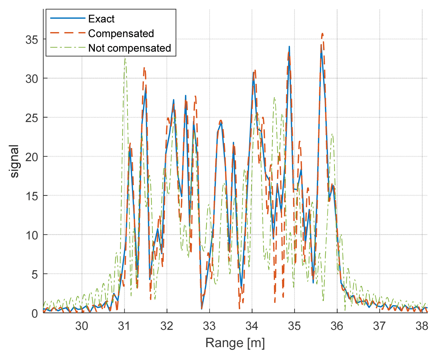
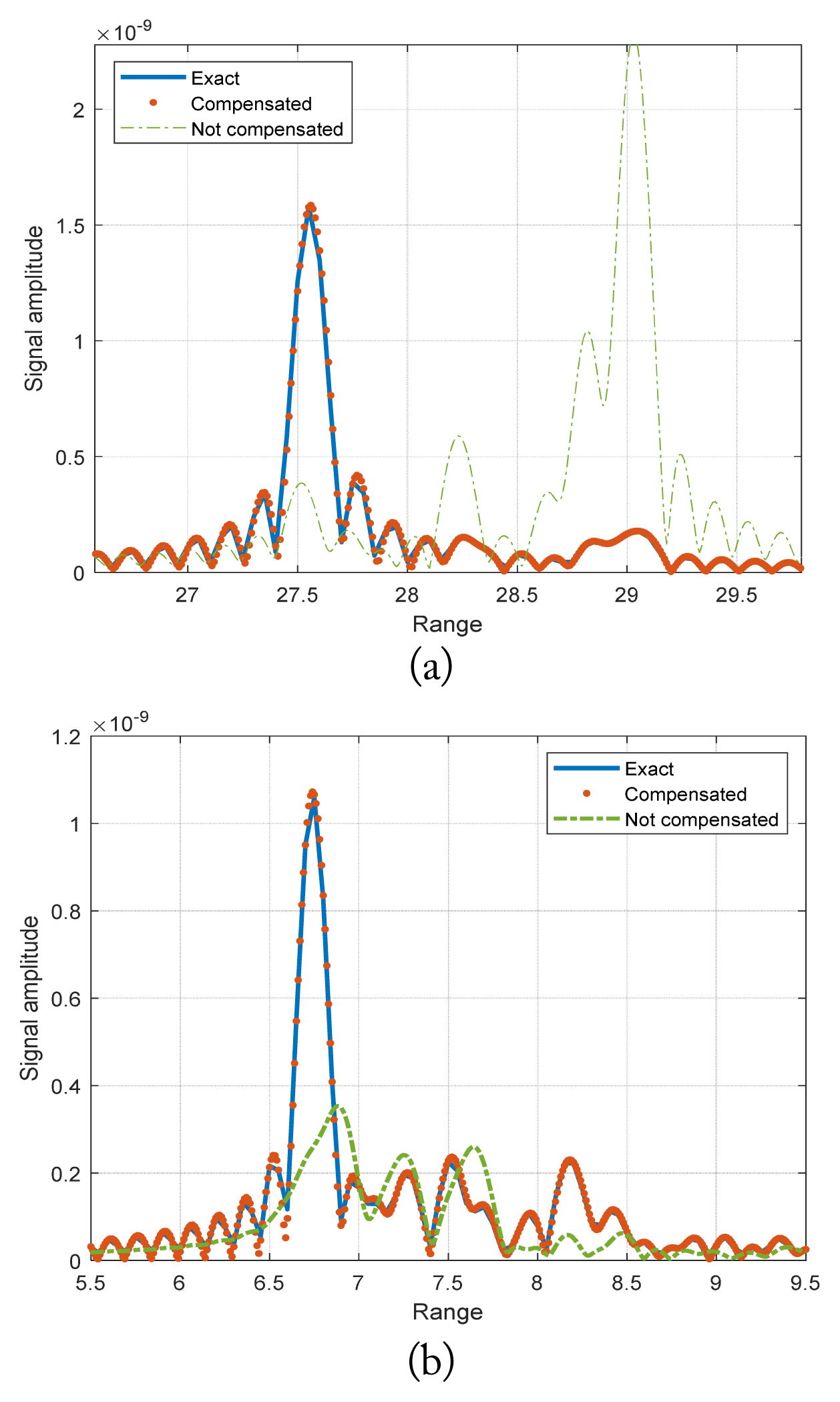
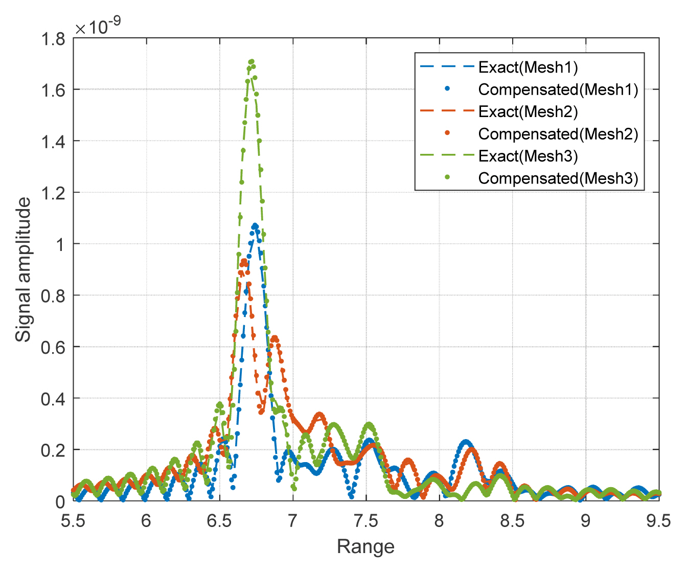
First, the proposed echo signal generation scheme is numerically verified for two cases: randomly distributed point targets and a moving vehicle. Fig. 6 shows the time-domain echo signal from 10,000-point targets that are randomly located between 31 m and 36 m away from the radar. The range bin size is assumed to be 1 cm, so impulses return from around 20-point targets in one range bin on average. The exact calculation of the echo signal, Eq. (6), is compared with the approximated Eq. (12) with and without the phase compensation, Eq. (9), in Fig. 6. The phase compensation scheme can decrease the error compared with that of the results without compensation. Table 1 shows the comparison of the computational time for the exact and approximate schemes, which also shows a significant improvement. For the second case, we consider the computation of the echo signal from the car model. The car is meshed into 770k, 440k, and 180k triangles called Mesh 1, Mesh 2, and Mesh 3, respectively. For Mesh 2 and 3, around 900 and 400 triangles are in one range bin on average, respectively, while there are 2000 for Mesh 1. In the simulation adopting the parameters in Table 2, a car moves away from the radar, so the radar beam illuminates the rear portion of the car. The other car positioned on (8.5, 3.2, 0) m moves toward the radar at the side lane, so the beam illuminates the front portion, as shown in Fig. 4. In each case, the incident angle on the target is calculated as 180┬║ and 20.63┬║ in the target vehicleŌĆÖs local coordinate system. Fig. 7 shows the comparison between the exact and approximated calculation of the radar echo signal for each scenario for Mesh 1. Fig. 8 illustrates the comparison of the return signal for three meshes and the 20.63┬║ incident angle. The proposed compensation scheme can provide much higher accuracy. Because the size of the triangle of Mesh 3 is large, the number of triangles in one range bin can be widely varied, which generates the amplitude of the impulse at a time point. Hence, some discrepancies for Mesh 3 can be observed, but with an increasing mesh number, the result converges.
The computational time for Fig. 7 is also compared in Table 1, which shows more than a 3,000-time improvement. Therefore, the proposed signal generation scheme can be applied to a real autonomous driving scenario, where the radar echo signal should be simulated over a long period when the relative positions of the radar and the target are varied.
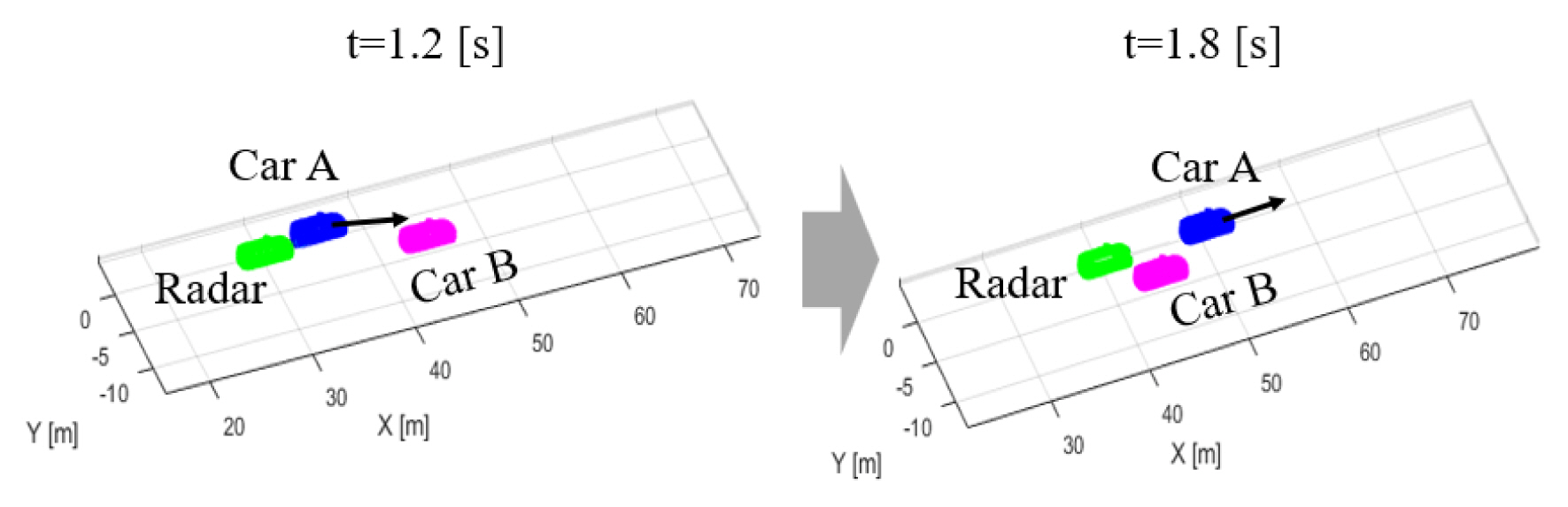
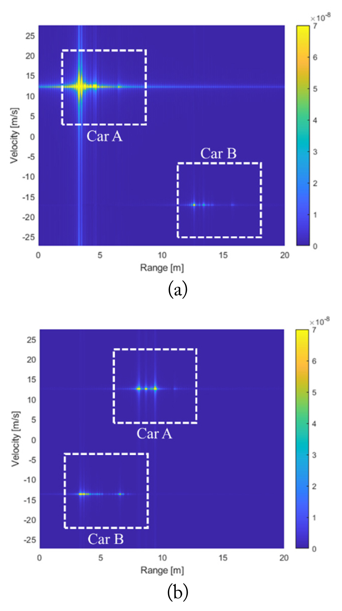
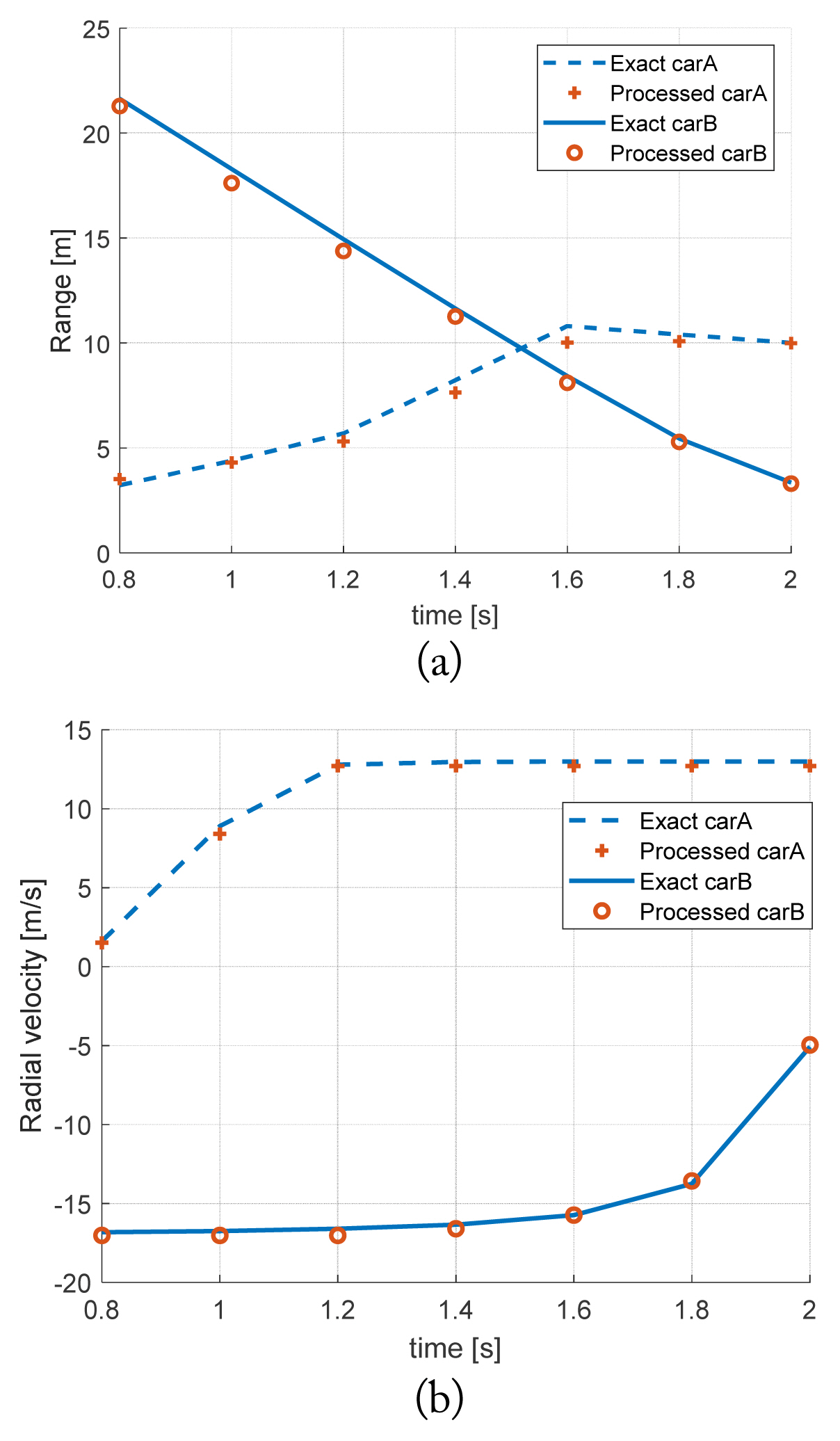
Next, the dynamic simulation is processed, which constructs several RD maps. For an autonomous driving simulation, we consider two moving cars and one stationary car: a car carrying the radar system, a moving Car A, and a stationary Car B. The simulation is performed from 0 to 2.8 seconds, which is divided into 15 stationary scenes per 0.2 seconds. The radar moves during the entire simulation time with a constant velocity, and Car A approaches and passes the radar from behind with a greater velocity than that of the radar. The radar keeps a line, while the Car A changes the line when it catches up with the radar. Fig. 9 shows the relative position among three cars at two timesteps, 1.2 and 1.8 seconds. In Table 3, the input values of locations and velocity are enumerated at two timesteps, 1.2 and 1.8 seconds. The other parameters are listed in Table 2. Based on the RD map, the range and relative velocity of two targets are calculated as Table 4. Fig. 10 shows the simulated RD map at 1.2 and 1.8 seconds, respectively. In Fig. 10, the vertical axis is converted from the Doppler frequency to the velocity with the relation of v = fD ╬╗/2. Based on Table 3, the exact range and velocity are calculated and compared with those from Fig. 10 in Table 4. Two estimations are in excellent agreement. Fig. 11 shows the comparison of the exact and the simulated range and the relative velocity for two cars from 0.8 to 2 seconds. The accuracy of the estimated results is very high. It takes 663 seconds to simulate the driving scenario with the 15 cuts. Therefore, the proposed scheme can be applied to a more general and complicated driving scenario.
IV. Conclusion
We have developed an autonomous driving simulator that can consider any scenario and arbitrarily shaped targets. To deal with the arbitrary shape, the first-order PO scheme is used to calculate the backscattering by the target, which discretizes the shape with many small triangular meshes. To efficiently calculate the echo signal from several meshes in the baseband, we approximate the impulse responses from the meshes with a phase compensation term and conduct the convolution of the approximated impulse response with the closed-form baseband signal representation of the radar system. Because the proposed scheme ignores the amplitude variation of the sinc function, the error of the return signal becomes large when the dimension of the mesh increases. If there are many small meshes in a range bin, the accuracy of the proposed scheme can be high, and the computational time is drastically reduced, e.g., over 3,000 times less for the considered case. Therefore, the proposed scheme is applied to a real driving scenario that repeatedly requires the computation of the time-domain echo signal for a varying relative position and velocity between the radar and the target. In a driving scenario, the radar system and one of the cars move along given paths, and the other car is stationary. The radar system is assumed to be a FMCW radar with a real RF specification. This scenario is simulated for a certain period to generate 15 RD maps. Based on the RD maps, the proposed simulator is numerically validated, and its accuracy is very high.