


I. Introduction
The finite-difference time-domain (FDTD) method [1ŌĆō4] has been popularly used for a variety of electromagnetic (EM) wave propagation phenomena in the EarthŌĆÖs atmosphere [5, 6]. The EarthŌĆÖs atmosphere consists of the troposphere, the stratosphere, and the ionosphere [7]. In the troposphere and stratosphere, only the refraction and attenuation phenomena affect EM wave propagation. However, EM wave propagation in the ionosphere is complicated because of various propagation environments, such as the static magnetic field of the Earth and plasma. Therefore, it is of great importance to accurately analyze EM wave propagation in the ionosphere modeled as anisotropic magnetized plasma. Plasma is a frequency-dependent dispersive medium, and it can be implemented in FDTD using various methods, such as the recursive convolution method [8], the Z-transform method [9], and the auxiliary differential equation (ADE) method [5, 6, 10]. The ADE-FDTD method is highly preferable because it involves a simple arithmetic implementation, and it can also be straightforwardly applied to nonlinear dispersive media, unlike other methods [11, 12]. There are two particular implementations in ADE-FDTD for the EM analysis of anisotropic magnetized plasma. First, the magnetic field (H) and the current density (J) are collocated at the same time step and position when discretizing J [5]; this is called the H-J collocated FDTD method. Second, the electric field (E) and J components are collocated at the same time step and position; this is called the E-J collocated FDTD method [6]. Unlike that of the H-J collocated method, the numerical stability condition of the E-J collocated method is independent of medium properties and remains the same as the Courant stability limit for free space [6]. Moreover, the E-J collocated method is more accurate than the H-J collocated method [6]. Note that unconditionally stable FDTDs for magnetized plasma have been proposed based on the weighted Laguerre polynomials [13] or the Crank-Nicolson-approximate-decoupling algorithm [14].
In FDTD, applying an appropriate boundary condition (ABC) to truncate the computational domain is necessary. Currently, the most efficient and commonly used ABC for FDTD is the perfectly matched layer (PML) [15, 16]. However, the PML implementation is not straightforward in the E-J collocated method, as a matrix calculation is involved in the FDTD update equations. To the best of our knowledge, the PML implementation to the E-J collocated FDTD scheme for anisotropic magnetized plasma has not yet been discussed. In this work, we propose a stable PML implementation suitable for the E-J collocated FDTD approach for anisotropic magnetized plasma. Toward this purpose, we employ complex stretching variables for the nabla operator when deriving FDTD update equations. Numerical examples are used to validate our proposed PML implementation.
II. Formulation
1. FDTD Update Equations
Let us consider the FDTD update equations for anisotropic magnetized plasma based on the E-J collocated method. The EM wave propagation in the anisotropic magnetized plasma region can be analyzed by MaxwellŌĆÖs equations coupled with the Lorentz equation of motion. The governing equation set is given by
where ╬Įc is the collision frequency, Žēp is the plasma frequency, Žēb is the cyclotron frequency, and ╔ø0 and ╬╝0 are the permittivity and permeability of free space, respectively. The cyclotron frequency is a function of the static magnetic field. Therefore, the cross-product term in Eq. (3) can lead to anisotropy of plasma so that the EM wave behavior depends on the direction of the static magnetic field relative to the EM wave propagation direction. In the E-J collocated method, the current density vectors are collocated at the same time step and position of the electric field vectors. Therefore, by applying the central difference scheme (CDS) in both time and space to Eqs. (1)ŌĆō(3), one can obtain the FDTD update equations consisting of three standard update equations for the magnetic field components and six coupled update equations for the electric field and current density components.
The update equations for Eq. (1) using CDS are as follows:
(4)
(5)
(6)
The update equations for Eq. (2) using CDS are as follows:
(7)
(8)
(9)
The update equations for Eq. (3) using CDS are as follows:
(10)
(11)
(12)
Here, the superscript and the subscript refer to the time and spatial indexing, respectively. The Žēbx, Žēby, and Žēbz are the cyclotron frequencies along each direction. As shown in Eqs. (7)ŌĆō(12), the update equations of E and J are required at the same time step, and thus the final FDTD update equations are expressed in a matrix form. For brevityŌĆÖs sake, we use the following notation:
(13)
(14)
(15)
where A[6 ├Ś 6], B[6 ├Ś 6], and C[6 ├Ś 6] are the coefficient marices that depend on the anisotropic magnetized plasma properties and the FDTD modeling parameters for time and space. It should be emphasized that the matrix calculation is performed only once before FDTD time marching, and thus the demanding computational cost is negligible. Note that there is a spatially non-collocated status of electric fields, magnetic fields, and current densities. To address this problem, we use the space averaging technique for all the spatially non-collocated components to maintain second-order accuracy [6]. For example, the final update equation of Ex for anisotropic magnetized plasma can be expressed as
(17)
where the superscript <a, b> refers to the corresponding index of the matrix element of [AŌłÆ1B] and [AŌłÆ1C]. In Eq. (17), the electric fields (E╠ā), magnetic fields (H╠ā), and current densities (J╠ā) should be considered by applying spatial averaging at position (i + 1/2, j, k) of the Ex field component. The other coupled components, Ey, Ez, Jx, Jy, and Jz, are obtained in a similar manner as Eq. (17). Note that the final update equations for the magnetic field component can be obtained through the standard FDTD process (Eqs. (4)ŌĆō(6)) because there is no field coupled with other field components.
2. PML-FDTD Update Equations
Let us consider the ABC for the E-J collocated FDTD method. In this work, the complex frequency-shifted (CFS)-PML is employed to prevent the spurious late-time growth of EM fields [16]. By using a modified nabla operator with complex stretching variables,
where a CFS stretching is utilized so that
Here, ╬Č = x, y, z. The CFS stretching (╬▒╬Č ŌēĀ 0) leads to a slightly more costly time-domain implementation than the standard PML stretching (╬▒╬Č = 0), but the former is more effective at absorbing evanescent waves and low-frequency fields, as it can correctly operate for Žē ŌåÆ 0. Except for considering ╬║╬Č variable, the update equations of the CFS-PML E-J collocated FDTD are almost the same as those of the E-J collocated FDTD based on Eqs. (7)ŌĆō(12). In general, PML implementation is straightforwardly applied to most FDTD update equations. However, it is not straightforward in the E-J collocated FDTD, as the current density components are collocated at the same time step and position of the electric field components. Therefore, the CFS-PML implementation is also included in matrix form for the update equations of the E-J collocated FDTD:
(20)
The final update equation of Ex for anisotropic magnetized plasma in the PML region can be expressed as
(22)
Here, fxy, fxz, fyz, fyx, fzx, and fzy are the auxiliary variables of CFS-PML implementations [17]. The auxiliary variables are given by
(25)
and Žā╬Č, ╬║╬Č, and ╬▒╬Č are the parameters related to the CFS-PML [16]:
where d is the thickness of the PML. The remaining auxiliary variables can be obtained similarly to Eq. (23) and Eq. (24). D[6├Ś6] is the coefficient matrix that depends on the modeling parameters. Similarly, the PML implementation should be considered for the other coupled components (Ey, Ez, Jx, Jy, and Jz) in the matrix of Eq. (20).
Before proceeding with the numerical examples, note that other PML implementation can be possible. Similar to conventional PML implementation, PML can be implemented by simply adding auxiliary variables. In this approach, the final update equation of Ex for anisotropic magnetized plasma in the PML region is expressed as
(29)
However, this conventional PML implementation in anisotropic magnetized plasma may lead to diverging FDTD results, which will be shown in the next section.
III. Numerical Examples
For simplicity, without loss of generality, the one-dimensional (1D) problem (along the z-axis) is considered for analyzing the EM wave interaction with anisotropic magnetized plasma. An x-polarized differentiated Gaussian pulse is considered in the 1D region of the anisotropic magnetized plasma region with an arbitrary angle ╬Ė (0┬░, 30┬░, 60┬░, and 90┬░) between the wavenumber vector and the DC bias magnetic field. The computational domain contains 500 cells with a uniform grid ╬öz = 75 ╬╝m and a temporal cell size ╬öt = 0.2475 ps. Ten cells of CFS-PML were used at the terminations of the space to eliminate unwanted reflections. The plasma parameters are modeled to have an electron density without ions under an applied 1.7 T magnetic field. Therefore, the electron plasma frequency Žēp = 2ŽĆ ├Ś 50 ├Ś 109 rad/s, the electron cyclotron frequency Žēb = 3 ├Ś 1011 rad/s, and the electron collision frequency vc = 20 ├Ś 109 Hz [18].
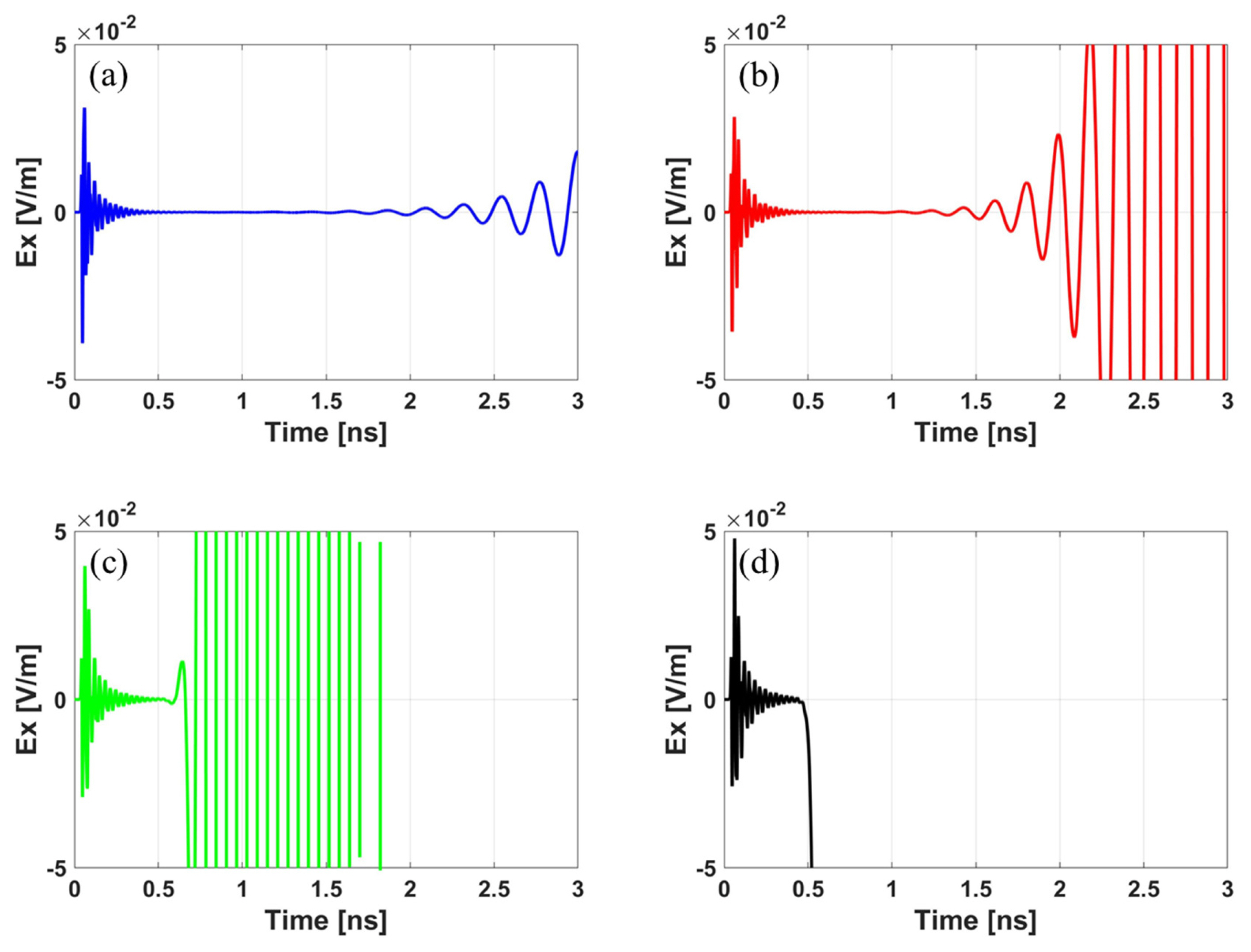
Let us consider the conventional PML implementation, e.g., (29). Fig. 1 shows the time-domain waveforms of the Ex field component at the observation point located 50 cells away from the source. As shown in Fig. 1, the conventional PML-FDTD simulation results are inaccurate and even divergent in all cases.
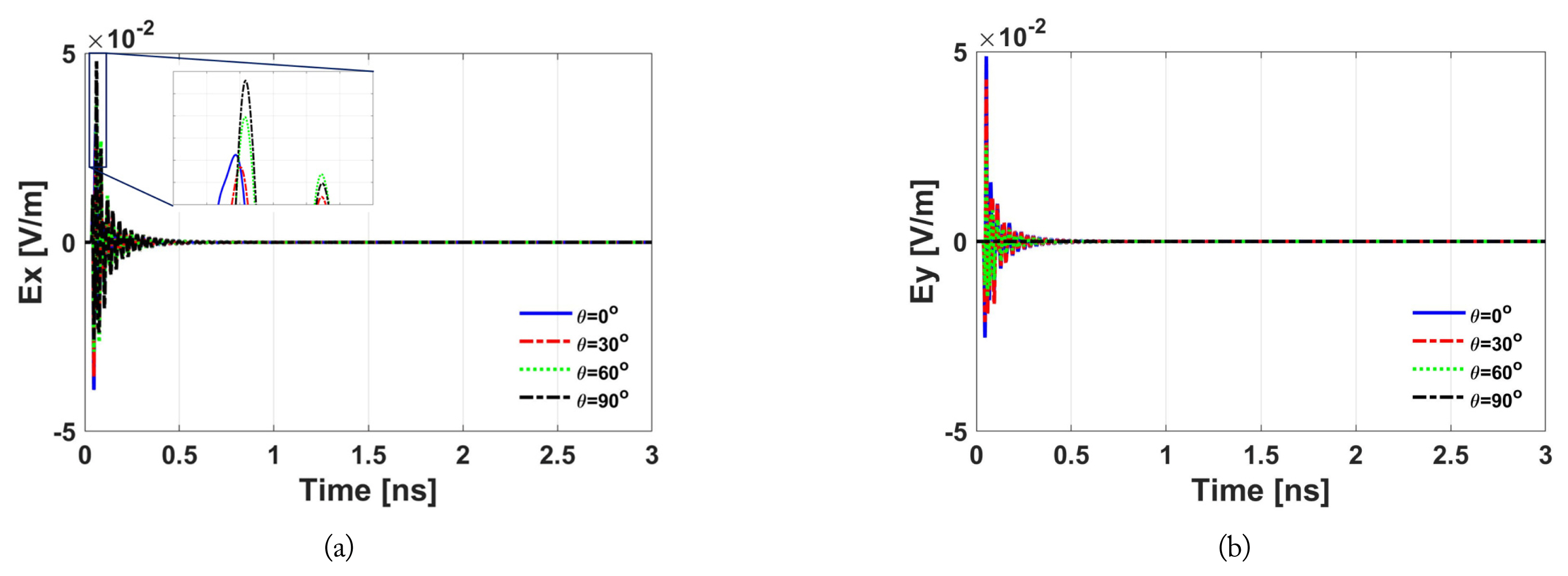
Now, let us consider the proposed PML implementation, e.g., (22). Fig. 2 shows that the FDTD simulation results are numerically stable in this case. As shown in Fig. 2, the Ey field component exists under the x-polarized incident field. This implies that the proposed FDTD algorithm can successfully analyze the anisotropic phenomenon of magnetized plasma.
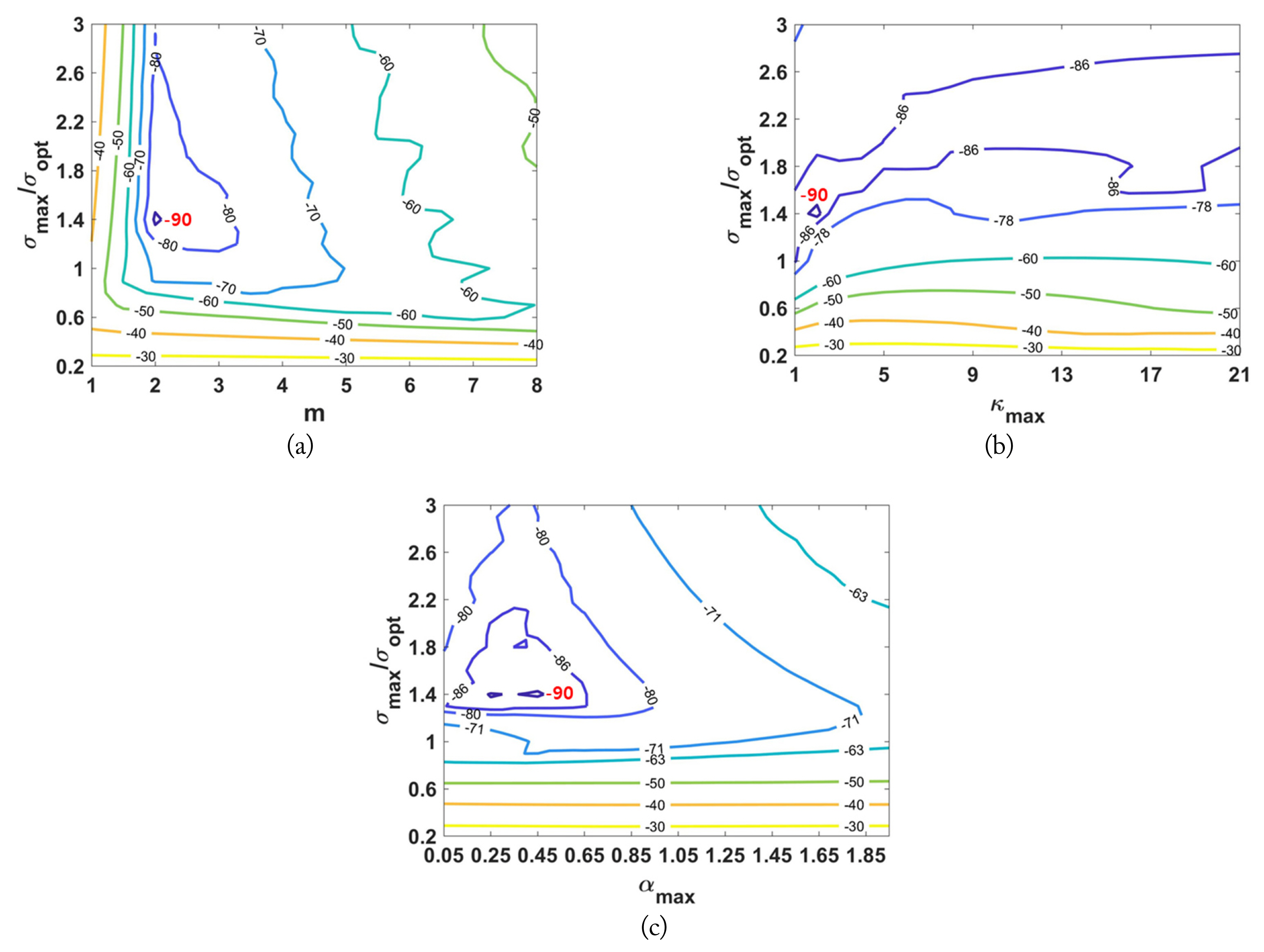
We then conduct a parametric study for the proposed PML performance. An angle between the wavenumber vector and the DC bias magnetic field is 0┬░. All the other parameters are the same as in the previous simulation. The reference solution is obtained using a large FDTD domain such that the reference solution is not contaminated by PML reflections [1]. The reflection error from the PML is defined as
where E(t) is the proposed PML implemented electric field, and Eref(t) is the reference electric field.
Here, Žāopt is scaled as follows [1]:
where ╬Ę0 is the free-space wave impedance, and ╬ö is the lattice-cell dimension. As shown in Fig. 3, the optimum CFS factors are m = 2, Žāmax/Žāopt = 1.4, ╬║max = 2, and ╬▒max = 2. These factors yield the lowest reflection error of ŌłÆ90 dB. We also compute the relative error for the optimum CFS factors under various DC bias magnetic fields. Fig. 4 shows that the PML performance is good, and thus the proposed PML implementation is suitable for the EM analysis of anisotropic magnetized plasma.
Finally, we compute the right-hand circularly polarized (RCP) and left-hand circularly polarized (LCP) reflection coefficients of the EM wave in the magnetized plasma slab with an arbitrary angle ╬Ė (0┬░, 30┬░, and 60┬░). The computational domain is divided into 500 cells, and the plasma slab occupies 120 cells. All the other parameters are kept the same as in the previous simulation. As shown in Fig. 5, the proposed E-J PML-FDTD simulation results have a good agreement with the analytic results [19].
IV. Conclusion
In this work, we have proposed a stable PML implementation suitable for the accurate FDTD method for the analysis of EM wave propagation in anisotropic magnetized plasma. Toward this purpose, we have developed an accurate E-J collocated FDTD algorithm for the plasma region with an arbitrary geomagnetic field by including the PML variables in the FDTD matrix update equations. The proposed PML-FDTD method can be applied to accurately predict EM wave propagation in the atmosphere for radio and satellite communication.