Calculation of Site Attenuation for Calculable Dipole Antennas
Article information
Abstract
This paper presents a method for calculating the site attenuation (SA) of an open-area test site (OATS) for a pair of calculable dipole antennas with a 3-dB hybrid balun in the frequency range of 30 MHz to 1 GHz. The SA was directly derived using the concept of power mismatch and dissipative loss from the SA measurement system instead of the concept of substitution loss. Two types of SA formulas using the power loss concept on the treatment of the OATS are presented. The first is the SA formula related to knowing only the value of the SA. The other is the SA formula that analyzed the effects of each part of the SA. Additionally, the constituent losses of the SA measurement system are discussed using the derived SA formula. The analysis of the results showed that the SA could be successfully characterized individually from the loss of the OATS. It also showed that SA is expressed as two kinds of losses: the balanced port-mismatch losses of transmit and receive baluns and the half-space dissipative loss. The resultant SA showed good agreement with the results calculated from the S-parameters as well as with the measured results.
I. Introduction
Site attenuation (SA) is a measure of the performance of an open-area test site (OATS) that is used to calibrate the electromagnetic compatibility (EMC) antennas for field strength measurements and radiated emission measurements [1–14]. An example of an OATS is the open-field EMC antenna calibration facility at the Korea Research Institute of Standards and Science. This facility has gained wide acceptance as a national standard for an open-field site.
The SA of an OATS is a measure of the transmission path loss of the space with a ground plane (open-field site or half-space) between the transmit (TX) and receive (RX) antennas. Many researchers have reported various approaches for theoretical calculations of SA [2–14]. Most of the research into SA calculation has employed the concept of insertion loss (known as a substitution loss [15]) with and without considering the test site. However, the effects of including antenna baluns and cables cannot be considered individually from the loss of the half-space and all other parts because all these effects are incorporated in the concept of SA. Calculable dipole antennas have also been developed and used as standard antennas [13, 14, 16–18]. For example, Salter and Alexander [13, 14] analyzed insertion loss for calculating the SA using a two-port model and the scattering parameters of a calculable standard dipole antenna.
The authors [19] directly derived a new equation for the SA measurement system without using substitution loss. Their SA measurement system included TX and RX antennas (i.e., calculable dipole antenna with a 3-dB 180° hybrid balun in the frequency range of 30 MHz to 1 GHz). The equation was derived using the concept of power mismatch and dissipative loss, which was used to perform an error analysis of the SA [4] and an antenna factor calculation [16, 20]. The authors calculated only the value of the SA using the concept of power loss to calculate the SA of a calculable dipole antenna [19].
This paper extends and clarifies two types of SA formula using the concept of power loss for the treatment of the OATS. The first is an SA formula related to knowing only the value of the SA. The other is an SA formula that analyzes the effects of each part of the SA. Additionally, the constituent losses of the SA measurement system are discussed in detail using the derived SA formula. The analysis of the results showed that the SA of the OATS can be successfully characterized individually from the SA measurement system and that the SA is expressed as two kinds of losses: the balanced port-mismatch losses of the TX and RX baluns and the half-space dissipative loss. This paper deals only with the classical SA. The resultant classical SA was in good agreement with the results derived from the S-parameters using the substitution loss, and with the measured results [13].
II. Analysis of the Site Attenuation Measurement System
1. Total Power Losses
Fig. 1 shows the configuration of the SA measurement system using calculable dipole antennas with a 3-dB hybrid coupler and two phase-matched coaxial lines on the OATS. Two dipole antennas were located along the x-axis (horizontal polarization, HP) or the z-axis (vertical polarization, VP) above a ground plane. The height of the TX antenna was h1, and the height of the RX antenna was h2. Additionally, d was the distance between the TX and RX antennas.

Site attenuation measurement system. Antennas are placed horizontally or vertically.
Fig. 2 details the power mismatch and dissipative loss factors of the SA measurement system, as well as the basic structure of the calculable dipole antenna with a 3-dB hybrid coupler and two phase-matched coaxial lines that were used in the SA measurement. The dipole antenna had a length of L and a radius of a. The balun was designed such that its complex S-parameters could be easily measured. Two semi-rigid cables with a length of LB from the 3-dB hybrid coupler were connected to the antenna terminal, as shown in Figs. 1 and 2. A 50-Ω load was connected to the sum port (Σ) of the hybrid, and a matched measuring instrument was connected to the other port (Δ) using a coaxial cable with a length of L2. The inner conductors of the two semi-rigid cables were connected to the balanced dipole elements, while the outer conductors were in contact with each other electrically (i.e., short-circuited at the feeding point of the dipole elements). Since this structure was perfectly symmetrical, the two matched output voltages of the balun had the same amplitude and a phase difference of π radians. The details of calculable dipole antenna analysis using the concept of power mismatch and dissipative loss are given in [4, 15, 18].
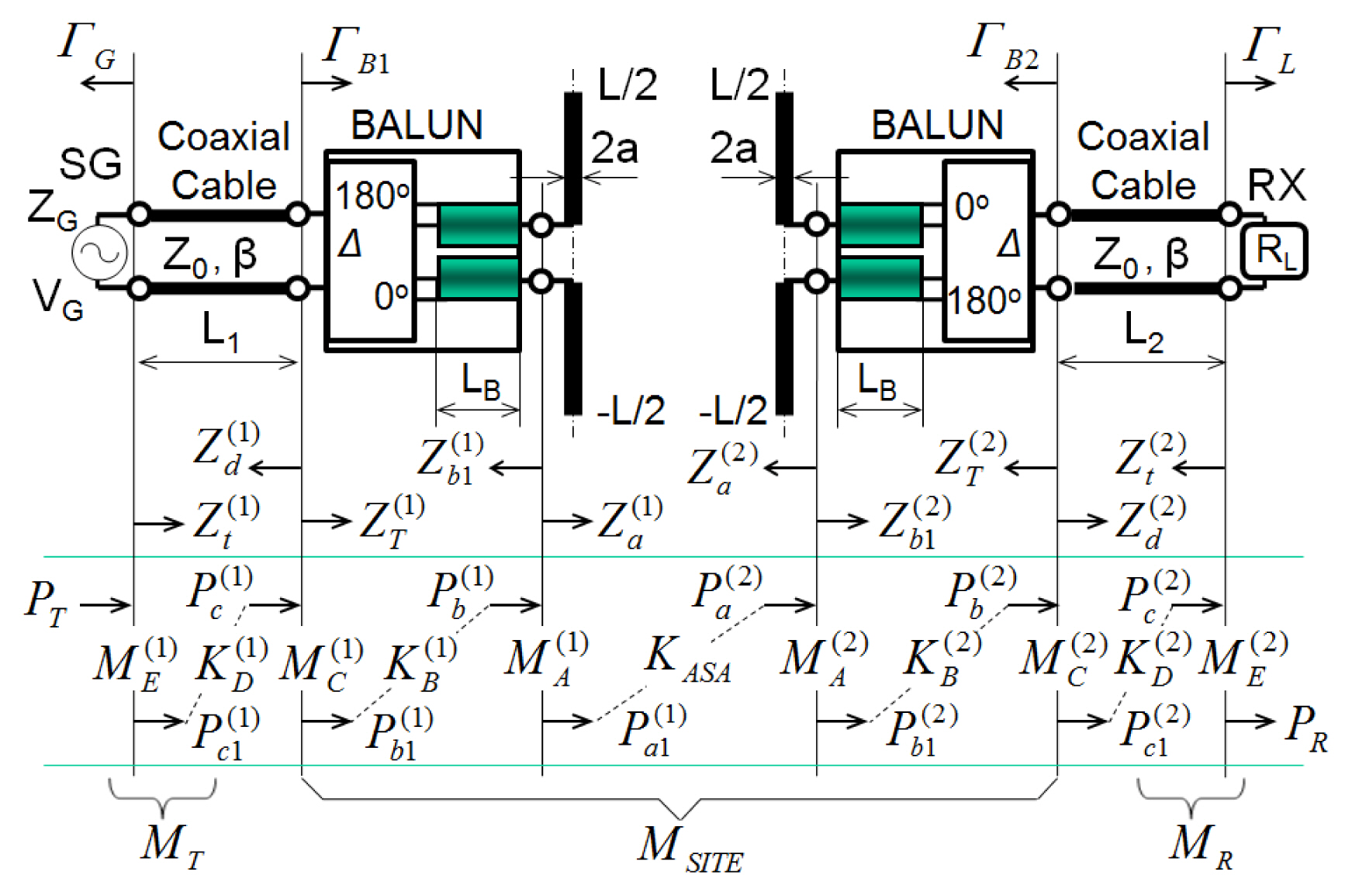
Site attenuation measurement system.
The TX antenna was excited by a signal generator (SG) through a coaxial cable, and the 3-dB hybrid coupler and RX antenna received the signal radiated by the TX antenna through the OATS, as shown in Fig. 2. The SA accounted for all power losses occurring between the RX and TX antennas over the ground plane. Two kinds of losses generally occur: conjugate mismatch losses and dissipative losses. Mismatch losses occur at the inputs and outputs of the hybrid baluns, the output of the SG, and the input of the receiver—details shown in Eqs. (4a), (4c), (4e), (4g), and (10). Dissipative losses occur in the cables, the hybrid baluns (Eqs. (4b), (4f), and (11)), and the half-space (Eqs. (4d)). The power losses experienced by the SA measurement system can be represented individually by these mismatch and dissipative losses. Each parameter referenced in Fig. 2 is listed in Table 1.

List of each parameter
Assuming only passive devices existed between the SG and the measuring receiver, the total power losses can be represented as follows:
where MT and MR are the power mismatch and dissipative losses in the TX part (SG–coaxial cable) and the RX part (coaxial cable–receiver), respectively, and MSITE denotes the power mismatch and dissipative losses of the site with a ground plane between the two antennas that included the baluns. In comparison to MT and MR, the site power loss MSITE was significantly large.
2. Site Attenuation
SA is defined as the minimum site power loss between the two antennas including the baluns obtained as the RX antenna scans over a given range of height values. The commonly used ranges of h1, h2, and d in the SA calculation are listed in Table 2 [1]. For the given values of d, h1, and h2, the theoreticcal SA of the OATS was defined from MSITE as follows:

Values used for calculating site attenuation (unit: m)
where MSITE is the minimum value of the power loss.
where
and
To evaluate Eqs. (5a) and (5b), the method of moments (MoM) has been widely used [12, 16, 17, 21]. In this study, the piecewise sinusoidal basis function with a Galerkin procedure was employed.
Since the hybrid balun had a 100 Ω balanced port and 50 Ω unbalanced port [13], the
Substituting Eqs. (4c)–(4e) into Eq. (6), the SA in decibels can be expressed in a simplified form as follows:
SA can be determined even if only Eq. (7) is used. However, employing the Eqs. (3) and (6) is useful for analyzing the effects of each part of the SA. Eq. (14) (see below) can also be used to consider the constituent losses of the SA measurement system and thus considering the two types of SA expression.
3. Power Losses on the Coaxial Cables
To consider all the constituent losses of the SA measurement system, MT and MR must be evaluated. The power losses on the coaxial cables connected to the SG and receiver are expressed as follows:
where the respective mismatch losses are given as follows:
and the dissipative losses are as follows:
In Eqs. (10) and (11),
The individual impedances of each section are as follows:
and
where
III. Calculated Site Attenuations
The calculated results showed that the SA of Eq. (3), which was derived from the concept of power mismatch and dissipative loss, produced the same result as that of the SA derived from the S-parameters by the National Physical Laboratory (NPL) [13].
To calculate the SA, a thin-wire kernel approximation with a segment length of 0.0125λ was used for the piecewise sinusoidal Galerkin’s MoM analysis. The dipole radius (a = 3.175 mm; 30 MHz ≤ f < 300 MHz and a = 0.794 mm; 300 MHz ≤ f < 1 GHz) was chosen to be less than 0.007λ (thin-wire approximation), and a nominal value of 50 Ω was used for the characteristic impedance Z0. A coaxial cable (RG-214/U; the velocity of propagation was 66% of the velocity in free space; dielectric constant, ɛr = 2.3) with a length of 10 m was selected for the numerical calculation. This cable had an attenuation of 0.049 dB/m at 50 MHz, 0.069 dB/m at 100 MHz, 0.165 dB/m at 500 MHz, and 0.269 dB/m at 1,000 MHz [22].
To validate the theoretical analysis, the SA results were compared with the results of the experiments [13], as shown in Table 3. Table 3 also shows the SA calculated by the NPL using the S-parameters [13]. In [13], MININEC was used for the dipole length and the antenna calculations, while the present study employed the piecewise sinusoidal basis functions with a Galerkin procedure. The difference between the calculated and MININEC SA was less than 0.09 dB, excepting 866 MHz. Additionally, the difference in the dipole length was less than 0.007λ for the seven frequencies. These differences were due to the differences in the basis functions.

Measured and calculated site attenuation SA; d = 10 m, h1 = 2 m
The results showed that the calculated SAs obtained using the power mismatch and dissipative loss concept were in good agreement with the results derived from the S-parameters as well as with the experiments.
Fig. 3 shows the frequency characteristics of the theoretical SA for the horizontal and vertical polarizations at given distances of 3 m, 10 m, and 30 m. The detailed values of the SAs calculated in this paper are shown in Tables 4, 5, and 6. In these Tables, the resonant dipole lengths for a calculable dipole antenna with a 3-dB hybrid balun at the frequency range of 30 MHz to 1 GHz are shown for the 24 individual frequencies. The heights of the RX antenna and the minimum attenuation at the given distances and frequencies are also shown.

Calculated site attenuations for the horizontal polarization (a) and vertical polarization (b).
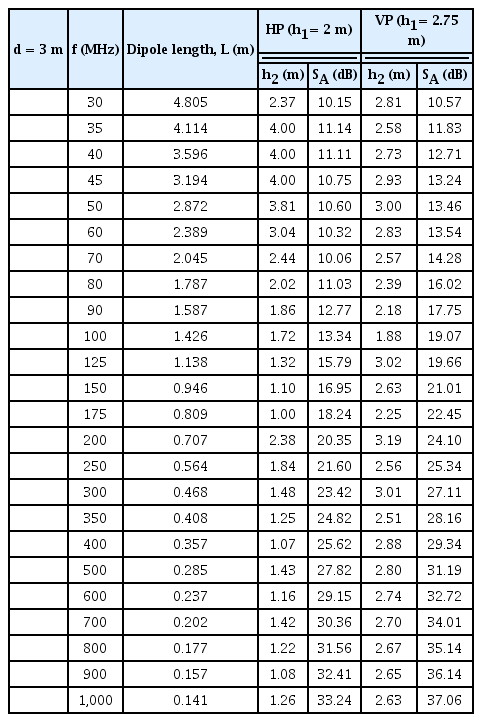
Calculated site attenuation SA for d = 3 m

Calculated site attenuation SA for d = 10 m
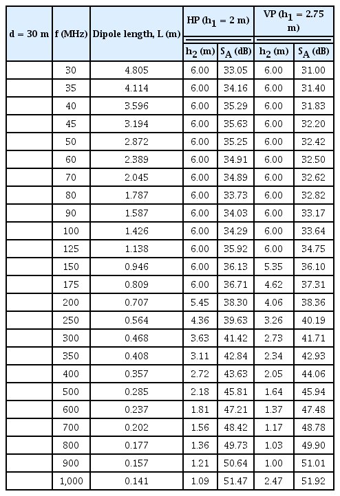
Calculated site attenuation SA for d = 30 m
The results of the calculated SA shown in Tables 4, 5, and 6 were compared to the results of the S-parameters expression given in [13]. The calculated SAs were better matched to the S-parameter SA as the distance between the TX and RX antennas increased. However, in the low frequency range of 30–90 MHz at the 3-m distance, the differences between the calculated SA and the S-parameter SA were greater but still less than ±0.73 dB. This difference was thought to be due to how the conversion errors of the impedance- and S-parameters affected the height pattern of the RX antenna under the strong mutual coupling of the antennas and ground plane. However, more research is needed.
IV. Constituent Losses for the Site Attenuation Measurement System
As shown in Eq. (1), the total power losses of the SA measurement system for the OATS with a pair of calculable dipole antennas with a 3-dB hybrid balun consisted of MT, MR, and MSITE. In other words, the total power loss of the SA measurement system consisted of a combination of the TX part (SG–coaxial cable) and the RX part (coaxial cable–receiver) of the power mismatch and dissipative losses in the open-field site transmission path loss MSITE as follows:
where ST and SR are the power losses (mismatch and dissipative losses) of thse TX and RX parts at a minimum site transmission path loss, respectively.
The total power losses of the SA measurement system are tabulated (in dB) in Table 7 for several different frequencies using the 3-m distance as an example. As indicated by the data in Table 7, the SA of an OATS can be characterized individually from the loss of the OATS and all other parts using the power mismatch and dissipative loss factors. Also, ST and SR were calculated to be in the order of 0.490 to 2.690 decibels; hence, ST+SR < SA. Therefore, the site power loss MSITE was significantly large.

Calculated mismatch and dissipative losses of the SA measurement system for d = 3 m
As mentioned previously, since the hybrid balun had a 100 Ω balanced port and 50 Ω unbalanced port [13], the
Fig. 4 shows the mismatch loss

Calculated mismatch loss
As shown in Fig. 4, for the 30-MHz HP at the 3-m distance (the worst case of the three distances), the mismatch loss
The average value of the mismatch loss (
As a result, the half-space dissipative loss KASA was the dominant component in the SA, because the mismatch loss
V. Conclusion
The two types of SA formulas for an OATS were presented using the power loss concept for the SA measurement system directly without the use of a substitution loss. Additionally, the constituent losses of the SA measurement system were considered using the derived SA formula. The analysis of the results showed that the SA of the OATS could be successfully characterized individually from the SA measurement system and that the SA is expressed as two kinds of losses: the balanced port-mismatch losses of the TX and RX baluns and the half-space dissipative loss. This approach enables the separation and analysis of the SA’s constituent power losses. It may also be useful for further studies on uncertainty evaluation. This paper deals only with the classical SA; the normalized SA will be presented in a future study.
Acknowledgments
This work was initially based on the KRISS/University cooperative research program. This work was also partially supported by the 2016 Yeungnam University Research Grant.
References
IEEE Standard for Methods of measurement of radio-noise emission from low-voltage electrical and electronic equipment in the range of 9 kHz to 40 GHz, ANSI C63.4-2003. 2004
Biography

Ki-Chai Kim received the B.S. degree in electronic engineering from Yeungnam University, Korea, in 1984, and the M.S. and Dr. Eng. degrees in electrical engineering from Keio University, Japan, in 1986 and 1989, respectively. He was a senior researcher at the Korea Standards Research Institute, Daedok Science Town, Korea, until 1993, where he worked in electromagnetic compatibility. From 1993 to 1995, he was an Associate Professor at Fukuoka Institute of Technology, Fukuoka, Japan. Since 1995 he has been with Yeungnam University, Gyeongsan, Korea, where he is currently a Professor in the Department of Electrical Engineering. He received the 1988 Young Engineer Awards from the Institute of Electronics, Information and Communication Engineers (IEICE) of Japan and received Paper Presentation Awards in 1994 from the Institute of Electrical Engineers (IEE) of Japan. Additionally, Prof. Kim served as President of the Korea Institute of Electromagnetic Engineering and Science (KIEES) in 2012. His research interests include EMC/EMI antenna evaluation, electromagnetic penetration problems in slots, and applications of electromagnetic field and waves.

Hyuk-Jun Seo was born in Daegu, Korea, in 1980. He received the B.S. degree in electronics and computer engineering from Kyungpook National University, Daegu, Korea, in 2006, as well as the M.S. degree in engineering science from the University of Mississippi, MS, USA, in 2010. He is currently working toward the Ph.D. degree at Yeungnam University, Korea. From 2011 to 2013, he was a Junior Research Engineer at the Mobile Communication Advanced Product Research Institute of LG Electronics Inc., Seoul, Korea. Since 2014, he has been a Research Engineer at the Medical Device Development Center, Daegu-Gyeongbuk Medical Innovation Foundation (DGMIF), Daegu, Korea. His research interests include the design of EMC/EMI antennas, EMC test standards, and validation of the test site.

Tae-Weon Kang was born in Andong, Korea, in 1966. He received the B.S. degree in electronic engineering from Kyungpook National University, Daegu, Korea, in 1988 and M.S. and Ph.D. degrees in electronic and electrical engineering from Pohang University of Science and Technology, Pohang, Korea, in 1990 and 2001, respectively. In 1990, he joined the Korea Research Institute of Standards and Science, Daejeon, Korea, where he is now the Head of Center for Electromagnetic Waves and the principal research scientist working on electromagnetic metrology. In 2002, he spent a year as a Visiting Researcher under the Korea Science and Engineering Foundation postdoctoral fellowship program at the George Green Institute for Electromagnetics Research, University of Nottingham. There, he worked on measuring the performance of electromagnetic absorbers and on a generalized transmission line modeling method. His research interests include electromagnetic metrology, such as electromagnetic power, noise temperature, and antenna characteristics, and numerical modeling in electromagnetic compatibility.

Jae-Yong Kwon received the B.S. degree in electronics from Kyungpook National University, Daegu, in 1995, and the M.S. and Ph.D. degrees in electrical engineering from the Korea Advanced Institute of Science and Technology, Daejeon, Korea, in 1998 and 2002, respectively. He was a Visiting Scientist at the Department of High-Frequency and Semiconductor System Technologies, Technical University of Berlin, Berlin, Germany, in 2001 and at the National Institute of Standards and Technology (NIST) in Boulder, CO, USA, in 2010. From 2002 to 2005, he was a Senior Research Engineer at the Devices and Materials Laboratory, LG Electronics Institute of Technology, Seoul, Korea. Since 2005, he has been a Principal Research Scientist with the Division of Physical Metrology, Center for Electromagnetic Metrology, Korea Research Institute of Standards and Science, Daejeon. Since 2013, he has been a Professor in Science of Measurement with the University of Science and Technology, Daejeon, Korea. His current research interests include electromagnetic power, impedance, and antenna measurement. Dr. Kwon is an IEEE Senior Member and IEICE member.

Jeong-Hwan Kim was born in Cheongju, Korea in 1954. He received the B.S. degree in electrical engineering from Seoul National University, Seoul, Korea in 1978, and the M.S. and Ph.D. degrees from the Korea Advanced Institute of Science and Technology, Seoul, Korea in 1980 and 2000, respectively. Both degrees were in electrical and electronic engineering. He joined the Center for Electromagnetic Wave of the Korea Research Institute of Standards and Science, Daejeon, Korea in 1981. Since then, he has been working on developments of the six-port automatic network analyzer systems, standard antennas, and electromagnetics measurement standards.