A Simple Empirical Model for the Radar Backscatters of Skewed Sea Surfaces at X- and Ku-Bands

Article information

Abstract

I. Introduction

The radar remote sensing of the sea status is crucial for weather forecasting, navigation, and scientific studies. Radar backscatter from the ocean surface depends on the surface roughness and the dielectric constant of the water, in which the roughness of the sea surface mainly depends on wind speed and wind direction [1]. The measurement and characterization of the sea surface roughness is difficult, and so is the computation of the backscattering coefficient of a sea surface.

The backscattering coefficients of various sea surfaces were measured using spaceborne and airborne scatterometers [2–4]. The satellite synthetic aperture radar systems also provided a tremendous amount of radar backscatter data for various frequencies, angles, polarizations, and wind vectors [5–7]. Owing to the difficulty of theoretical modeling, attempts have been made for empirically modeling the backscattering coefficient of sea surfaces based on the radar measurements for various wind speeds and wind directions, the so-called “geophysical model functions (GMF)” such as SASS-2 for Ku-band [8], XMOD2 for X-band [7], CMOD5 for C-band [9], and L-GMF for L-band [6]. These empirical models are based on the functional form of σ ⁰=A+Bcosφ+Ccos2φ, where φ is the azimuth angle of the wind direction relative to the radar look direction. The coefficients A, B, and C of each GMF model are determined empirically based on the experimental data sets for each frequency band as functions of radar parameters (frequency, angle, and polarization) and wind speed. However, each of these empirical models has limited ranges of frequencies, polarizations, incidence angles, and wind vectors.

To obtain a wider validity region of a radar scattering model for various radar and sea-surface parameters, theoretical models of the backscattering coefficients for sea surfaces were developed on the basis of the approximated surface roughness characteristics and the integral equation method (IEM) model [10–13]. Surface roughness moments are related to its second-order and third-order cumulant functions known as correlation and bicoherence functions, respectively. The Fourier transforms of the correlation and bicoherence functions are the roughness spectrum and bispectrum. The sea surface can be modeled as a time-varying, anisotropic, and skewed rough surface, in which “skewness” is defined by the difference in the backscattering coefficients between the upwind (φ=0°) and downwind (φ=180°) directions, and “peakedness” is defined by the difference between the upwind (φ=0°) and crosswind (φ=90°) directions.

The surface skewness is described by the bicoherence or the bispectrum. Then, the backscattering coefficient of a sea surface can be estimated by adding a term associated with the roughness spectrum (correlation function) and the other term with the bispectrum (bicoherence) [1, 10]. The first term can be obtained by the traditional IEM, with the roughness spectrum corresponding to a correlation function with a root-mean-square (RMS) height and a correlation length. The second term may be obtained with a complicated bispectrum computation for the skewness effect. The bispectrum calculation involves one unknown parameter s ₀ (skewness factor) that may be empirically determined for a given wind speed.

To avoid computing the complicated bispectrum function B(k)=B _S (k)+jB _a (k) with an unknown parameter (skewness factor), which should be empirically determined for each wind speed, we attempted to generate an empirical expression for representing the skewness effect. In the computation of the first term of the theoretical model [10] associated with the correlation function, the correlation length of a sea surface is represented by the function of the correlation length of the upwind (L _u ) and crosswind (L _c ) directions and the azimuth angle of wind direction φ. We found that the correlation length could also include the skewness effect without the complicated second term when the correlation length is multiplied by a Gaussian-type functional form of the wind azimuth angle φ. In other words, the skewness effect can be practically accounted for by controlling the correlation length of a sea surface. The coefficients of the new multiplying function can be obtained by comparing the new model with an extensive experiment database. Unlike the existing model, which is complicated and has skewness factors that are determined for each wind speed, this new model is simple without the complicated bispectrum function and needs only the empirical determination of the coefficients for each frequency and polarization for a wide range of wind speeds. The accuracy of this new model was verified with the extensive experiment database at X-band. Surprisingly, the model agreed well with the Ku-band independent radar measurements [14].

II. The Existing Model

The IEM model has been widely used for estimating the backscattering coefficients of rough surfaces including rough sea surfaces [11]. The IEM model was applied to the measurement data in [2, 4] at X- and Ku-bands for VV and HH polarizations for various wind speeds and incidence angles using a simple exponential correlation function [11]. The IEM consists of two parts: σpp0=σpp0(N)+σpp0(S) , where the first part represents the backscattering coefficients of the non-skewed surfaces, and the second part represents the skewness effect.

where I _pp , W(K, φ), f _pp , F _pp , and B(K,φ) are given in [11], k ₁ is the wavenumber, θ is the incidence angle, and h _rms is the RMS height of a sea surface. The W ^{( n )}(K, φ) is the n ^th -order surface roughness spectrum, which is the Fourier transform of the n ^th -power of a correlation function. For an exponential correlation function, the roughness spectrum has the form of W ^{( n )}(K, φ)=nl _c [n ² +(Kl _c )²]^−1.5 with K=2k ₁ sinθ and l _c =L _u cos² φ+L _c sin² φ, where the correlation length l _c can be obtained from the upwind and crosswind correlation lengths, L _u and L _c , respectively, with the azimuth angle φ. The upwind and crosswind correlation lengths are given in [11] for the various wind speeds. As previously mentioned, a skewness factor s ₀ is used when describing the skewness effect. This constant is empirically determined at a wind speed, and thus it does not have the physical characteristics for wind speed. Moreover, Eq. (1b) is complicated, and the accessibility is poor. Therefore, we proposed a new simple model that does not need Eq. (1b) and has the physical characteristics for wind speed.

III. New Simple Empirical Model

In general, the RMS height and correlation length are mainly used to describe the roughness of a rough surface. As the roughness increases, the backscattering increases. As the RMS height increases and/or the correlation length decreases, the roughness increases. Therefore, if the correlation length decreases, the backscattering increases. We also used the roughness characteristic of the correlation length increasing in the order of upwind, downwind, and crosswind. Using these characteristics, we proposed a modified correlation length, which is the function of the azimuth angle. The peakedness and skewness of the backscattering coefficients at the azimuth angles of 0° ≤ φ≤ 360° can be controlled by the surface correlation length. Therefore, we proposed the following form of a modified correlation length with unknown constants: a, b, and c.

For example, Fig. 1 shows the typical angular responses of the backscattering coefficient σvv0(N) at a wind speed of 9.3 m/s, f=10 GHz, and θ=32° with various values of the unknown constants a, b, and c. The constant a in Eq. (2) mainly controls the skewness effect, as shown in Fig. 1—the solid line (a=0.5) and the dashed line (a=0.1) with fixed b and c. The comparison between the solid line (b=3) and the dotted line (b=1) shows that the constant b controls the peakedness (Fig. 1). The role of the constant c is mainly to control the level of the backscattering coefficient, as shown in Fig. 1—the solid line (c=0.7) and the dash-dot line (c=0.3) with fixed a and b. Therefore, the skewness and peakedness can be simply controlled by selecting the optimum values of a, b, and c.

Fig. 1

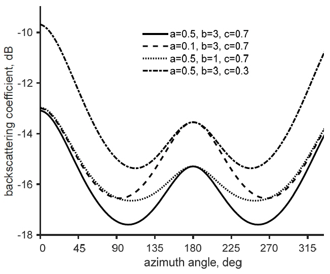
Backscattering coefficients σvv0(N) with various values of unknown constants a, b, and c.

We used measurement data [1] to propose the model using Eq. (2). The data used were measured in the sea near Japan and the Pacific Ocean using an airborne microwave scatterometer–radiometer system and showed how the backscattering coefficients changed for the wind direction. The backscattering coefficients were measured as combined functions of the microwave frequency (10.0 GHz and 13.9 GHz), polarization (VV and HH), incident angle (0°–70°), azimuth angle (0°–360°), and wind speed (3.2–19.4 m/s). In the data processing procedure for obtaining one point of data, the standard deviations for the wind direction were less than 1°, and the standard deviations for the backscattering coefficients were 0.3–1.0 dB.

An extensive database was obtained from [11] (originally [2, 4]), which consisted of 462 measurement data-points for VV and HH polarizations at various wind speeds (i.e., 3.2, 9.3, and 14.5 m/s at 10 GHz measurements at 32° and 52°, and 4.2, 5.5, 7.5, 12, 15, and 19.4 m/s for 13.9 GHz measurements at 40°). The optimum values of the unknown constants were obtained using the minimum root-mean-square errors (RMSEs) between the scattering model and the database as functions of wind speed u in the following forms:

If we use the correlation length using Eqs. (2) and (3), we can control the skewness effect without using the complex Eq. (1b). In the existing model, the skewness factor s ₀, which was obtained empirically for a wind speed, was applied, but the new model with (3) became much simpler because the correlation length is a function of wind speed. We can also predict the backscattering coefficients for continuous wind speeds.

IV. Verification of the New Model

To verify the accuracy of the new simple model that was empirically developed with Eqs. (2) and (3), we compared the new model with the existing model and the experimental datasets. For the existing model, the complicate skewness term σpp0(S) with the unknown skewness factor s ₀ was used. Conversely, the new model is simpler than the existing model for computing the backscattering coefficients of skewed sea surfaces.

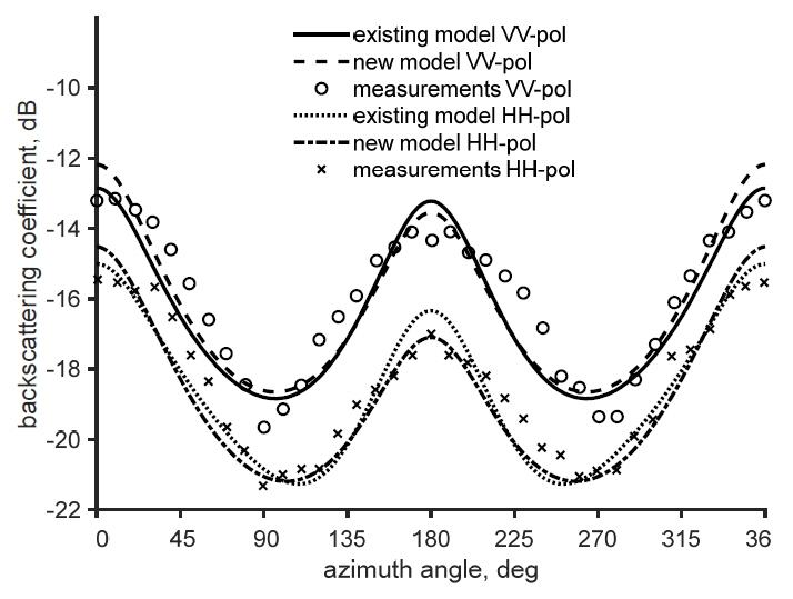
Figs. 2 and 3 show a typical comparison among the new simple empirical model, the existing model, and the measurement data. Both the new and existing models agree well with the measurements except for several points at the crosswind direction, as shown in Fig. 2. The accuracies of both models are comparable, as shown in Figs. 2 and 3.

Fig. 2

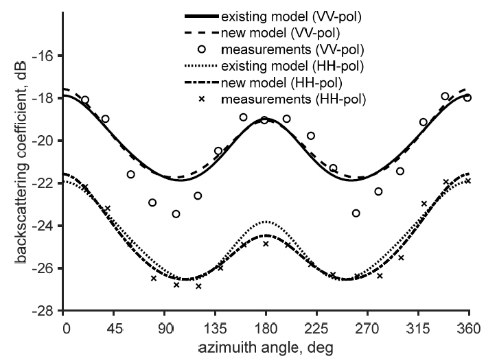
Comparisons between the existing model and the new model with 10 GHz measurements for a wind speed of 9.3 m/s at 52°.

Fig. 3

Comparisons between the existing model and the new model with 10 GHz measurements at 32° for VV-polarization (a) and HH-polarization (b).

Table 1 shows the RMSEs between the measurement data and the new model and those between the measurement and the existing model. For example, the RMSEs for the data at 10 GHz and 3.2 m/s for the VV polarization (crosses in Fig. 2) are 0.65 dB and 0.49 dB for the existing model and the new model, respectively, and for the data at 14.5 m/s (circles in Fig. 2), the RMSEs are 0.57 dB and 0.49 dB for the existing and new models, respectively, as shown in Table 1. Also Table 1 shows the comparable RMSE values for other datasets between the existing and the new model.

Table 1

RMSEs under various conditions

Fig. 4 shows the comparison of the new simple model with independent datasets [14] and the existing model. The RMSEs are the same at 0.71 dB for the existing and new models. The new empirical model agrees well with the experimental data, although the model is simpler than the existing model.

Fig. 4

Comparisons between the existing model and the new model with independent datasets acquired at 13.9 GHz for a wind speed of 12.8 m/s at 40°.

This new model has two main advantages over the existing model with comparable accuracies. First, this model is easily understandable and conveniently applicable because of its simplicity. Second, the calculation time is dramatically reduced with this new model. For example, when we compute the backscattering coefficients of sea surfaces for various conditions with 10 wind speeds, 360 wind directions, 90 incidence angles, 10 frequencies, and 2 polarizations (total of 6,480,000 data) using a personal computer, it takes only 73 seconds with this model and 7 hours with the existing model. In short, the calculation time is reduced to 1/345.

V. Conclusion

A new empirical scattering model for estimating the backscattering coefficients of skewed sea surfaces was proposed. This model is simpler and more practical than the existing model. Instead of using the complicated skewness term σpp0(S) , a modified correlation length was used in the new model to include the skewness and peakedness effects. The new simple empirical model agreed well with experimental datasets, and its accuracy was comparable with that of the existing model.

Article information Continued

References

Biography
Taekyeong Jin received the B.S. and M.S. degrees in electronic and electrical engineering from Hongik University, Seoul, Korea, in 2017 and 2019, respectively. He worked at the Hongik University Research Institute of Science and Technology, Korea, from March to June 2019. He joined Hanwha Systems in July 2019 as a Researcher. His research interests include microwave remote sensing, array antennas, and microwave scattering from sea surfaces.
Yisok Oh received the B.E. degree in electrical engineering from Yonsei University, Seoul, Korea, in 1982, the M.S. degree in electrical engineering from the University of Missouri, Rolla, MO, USA, in 1988, and the Ph.D. degree in electrical engineering from the University of Michigan, Ann Arbor, MI, USA, in 1993. In 1994, he joined the faculty of Hongik University, Seoul, where he is currently a Professor in the School of Electronic and Electrical Engineering. His current research interests include polarimetric radar backscattering from various Earth surfaces and microwave remote sensing of soil moisture and surface roughness.