An IE-FFT Algorithm to Analyze PEC Objects for MFIE Formulation
Article information
Abstract
An IE-FFT algorithm is implemented and applied to the electromagnetic (EM) solution of perfect electric conducting (PEC) scattering problems. The solution of the method of moments (MoM), based on the magnetic field integral equation (MFIE), is obtained for PEC objects with closed surfaces. The IE-FFT algorithm uses a uniform Cartesian grid to apply a global fast Fourier transform (FFT), which leads to significantly reduce memory requirement and speed up CPU with an iterative solver. The IE-FFT algorithm utilizes two discretizations, one for the unknown induced surface current on the planar triangular patches of 3D arbitrary geometries and the other on a uniform Cartesian grid for interpolating the free-space Green’s function. The uniform interpolation of the Green’s functions allows for a global FFT for far-field interaction terms, and the near-field interaction terms should be adequately corrected. A 3D block-Toeplitz structure for the Lagrangian interpolation of the Green’s function is proposed. The MFIE formulation with the IE-FFT algorithm, without the help of a preconditioner, is converged in certain iterations with a generalized minimal residual (GMRES) method. The complexity of the IE-FFT is found to be approximately O(N1.5) and O(N1.5logN) for memory requirements and CPU time, respectively.
I. Introduction
In this paper, we introduce a fast method of moments (MoM) [1] solution for three-dimensional (3D) perfect electric conducting (PEC) scattering problems. The electric field integral equation (EFIE) has been a popular choice. The solution derived from the EFIE has higher accuracy compared to that of the magnetic field integral equation (MFIE). However, the impedance matrix of MFIE has a better convergence rate when solved with an iterative solver. The traditional MoM solutions from the EFIE or MFIE suffer from prohibitive O(N2) complexities of memory requirements and CPU time to assemble the impedance matrix and perform the matrix-vector multiplication with an iterative matrix solver. For complex structures, the convergence of the impedance matrix is a big issue. Many researchers are interested in the MFIE formulation having better accuracy [2, 3].
For electrically large problems, several fast algorithms have been developed to overcome these numerical complexities. Multilevel fast multipole method (MLFMM) [4] is the most powerful algorithm, which has O(N) and O(NlogN) complexities for memory and the matrix-vector multiplication time, respectively. However, it has a strong dependence on integral kernels. There are several algorithms that are less kernel-dependent. The algebraic methods, such as IE-QR [5] and adaptive cross approximation (ACA) [6], have been developed to compress merely the impedance matrix. From the physical point of view, there are equivalent source approximations and Green’s function approximations, which are both employed on a uniform Cartesian grid. Among the equivalent source approximation methods, the precorrected fast Fourier transform (p-FFT) [7] and the adaptive integral method (AIM) [8] are the most well-known algorithms.
This paper extends an IE-FFT algorithm [9] into the MFIE formulation for 3D PEC geometries with closed surfaces. The IE-FFT algorithm uses algebraically simple Lagrange polynomials for the free-space Green’s function on a Cartesian grid. Through separation variables, the gradient of the Green’s function consists of one coefficient matrix and two Π matrices; one is for the integrand of the product of the curl of the basis functions and Lagrange polynomials, and the other is for the integrand of the cross-product of the basis functions and the gradient of the Lagrange polynomials. This results in a non-symmetric MFIE formulation. The proposed algorithm leads to O(N1.5) complexity for the memory requirement and O(N1.5logN) complexity for the matrix-vector multiplication. Even though the MFIE has an accuracy problem, it can yield reliable solutions with careful treatment.
This paper is organized as follows. Section II provides a description of the MFIE formulation. The detailed implementation of the IE-FFT algorithm is described in Section III. Through numerical examples, Section IV demonstrates the accuracy and performance of the proposed method. Finally, the paper is concluded in Section V.
II. MFIE Formulation
The MFIE formulation is briefly shown for an arbitrarily shaped 3D PEC object. The formulation is directly used in the computation of the near-field correction for the IE-FFT algorithm to ensure its accuracy. The MFIE formulation can be written from the boundary condition for the tangential magnetic field on closed surfaces as
To begin with, the discrete Galerkin statement for MFIE is shown below:
where Γh denotes the faceted surface of the PEC object, Xh is the finite dimensional trial and testing space, and λ⃗ (⇉) is the discrete Galerkin testing function.
The unknown current density induced on the surface is
where α⃗i(⇉) represents surface div-conforming Rao-Wilton-Glisson (RWG) vector basis functions [10]. The entries of the impedance matrix, Z, are given by
where
and
where N is the number of unknowns; note that supp() indicates the finite support of every non-boundary, edge-related basis function. Here, Dij and Pij are singular and coupling entries of the impedance matrix from the discrete Galerkin statement.
III. IE-FFT Algorithm
The IE-FFT algorithm makes a hexahedron bounding box that encloses the entire geometry in Fig. 1. A non-uniform triangular mesh for the RWG basis functions and a uniform Cartesian grid for the free-space Green’s functions are shown in two discretizations. Note that α is a constant used to define the near-field correction region, and λ is the wavelength. d is the sampling resolution. Here, L is the size of the second order Cartesian element.

Two discretizations for unknown current density and the free-space Green’s function.
The details of the IE-FFT algorithm are shown below.
1. A Uniform Cartesian Representation of Free-Space Green’s Function using Lagrange Polynomials
The free-space Green’s function is written in the matrix form:
where
and where the number of grid points is Ng =Nx × Ny ×Nz. Also, the dimensional indices could be expressed as n = (i, j,k) and n′=(i′,j′,k′) , where 0 ≤ i,i′< Nx , 0≤ j, j′ < Ny , and 0 ≤k k′, <Ny . The pth order interpolation basis functions,
The entries of G are the 3D block-Toeplitz matrix. Combined with Eqs. (6) and (8),
where gn,n ′ is the Lagrange coefficients of the free-space Green’s function. Interchanging summation and integration orders leads to
2. Representation of the Π Matrices
There are two projection matrices needed in the IE-FFT. They are:
and
respectively. In contrast to Eq. (3), ∇′g(⇉;⇉′) only depends on the Lagrange polynomials, i.e.,
where
The entries of Π⃗P are
where α⃗i,x (⇉), αi,y(⇉), and α⃗i,z(r⃗) are the vectors of the RWG basis function at the x-, y-, z-directions, respectively. Note that Π⃗p is a vector-valued and sparse matrix.
3. Near-Field Correction
In Fig. 1, the near-field interaction terms within αλ should be appropriately corrected to guarantee the accuracy. The correction entries are given as:
where 0 ≤i<N, j ∈ Lneig , and Lneig comprise the set of the near-field interaction elements.
4. Fast Matrix Vector Multiplication
The complexities of the Zcorr and Π matrices concerning the memory requirements and the matrix fill-in time are O(N). With the help of the FFT, the complexity of the matrix-vector multiplication of the G matrix leads to O(N1.5logN). The memory requirement of the G matrix is O(N1.5).
IV. Numerical Results
To demonstrate the efficiency of the proposed algorithm, a PEC sphere with a radius of 1.0 m is considered. The geometry of the PEC sphere is shown in Fig. 2. The triangular meshes are built so that there are at least λ/7. All numerical experiments are carried out on a 2 GB RAM Intel Pentium M processor 1.60 GHz. All computations have been performed in single precision arithmetic. Third-order Lagrange polynomials are used to interpolate the free-space Green’s function.
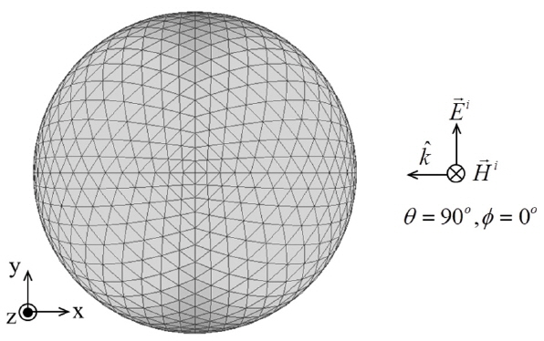
The geometry of a PEC sphere.
The results of the IE-FFT algorithm with the MFIE formulation are compared to those of the Mie series. Fig. 3 shows the results of the bistatic RCS at a frequency of 300 MHz. Three results of the Mie series, the conventional MoM, and the proposed approach are compared. In Fig. 3(a), the results between the Mie series and the MoM approaches are seen to be slightly different around 180°. However, the results between the traditional MoM and the IE-FFT algorithm have very good agreements on both the E-plane and the H-plane. Inaccuracy comes from the numerical integration in the hyper-singular part. The IE-FFT algorithm does not deteriorate the accuracy. The results of the bistatic RCS at a frequency of 600 MHz are shown in Fig. 4. The results from the Mie series and the IE-FFT algorithm also have reasonable agreements on both the E-plane and the H-plane. The largest difference between the two results is obtained around 160°–180° from the effects of the numerical integration. Fig. 5 shows the results of bistatic RCS at a frequency of 1,200 MHz. Both results are reasonable agreements.
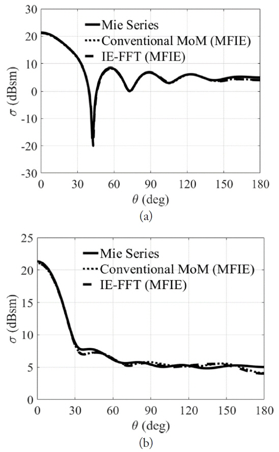
The bistatic RCS for a 1-m PEC sphere at a frequency of 300 MHz. (a) E-plane and (b) H-plane.
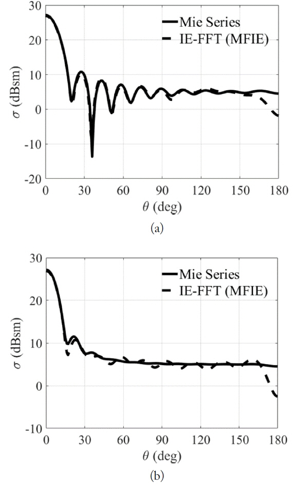
The bistatic RCS for a one-meter PEC sphere at a frequency of 600 MHz. (a) E-plane and (b) H-plane.
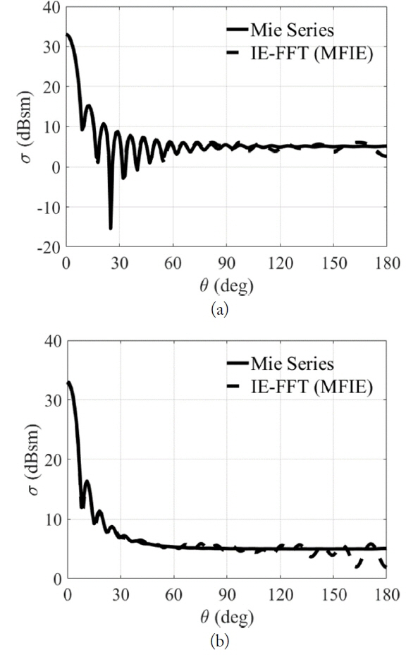
The bistatic RCS for a one-meter PEC sphere at a frequency of 1,200 MHz. (a) E-plane and (b) H-plane.
Table 1 summarizes the memory requirements of the IE-FFT algorithm for third-order Lagrange polynomials. All units are Megabytes. The memory of the correction matrix, Zcorr , and the Π matrices shows O(N) complexity. However, the coefficient of the free-space Green’s function is O(N1.5) complexity.
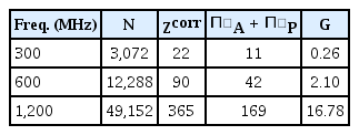
Memory requirement of the IE-FFT algorithm for scattering from a PEC sphere with a radius of 1 m
Table 2 summarizes the CPU time and the number of iterations of the IE-FFT algorithm with third-order Lagrange polynomials. The CPU time for the matrices fill-in has O(N) complexity. The CPU time for the matrix vector multiplication (MXV) is O(N1.5logN) complexity.
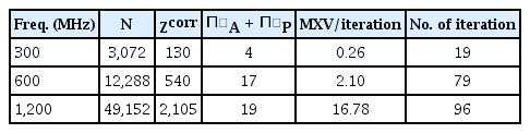
The CPU time and the number of iterations of the IE-FFT algorithm for scattering from a PEC sphere with a radius of 1 m
The memory requirement versus the number of unknowns is given in Fig. 6(a) for third-order Lagrange polynomials. The memory requirements of the correction, Π matrices, and the coefficients of the free-space Green’s function are plotted with circles, squares, and diamonds, respectively. The O(N) and O(N1.5) complexities are plotted as dashed and dotted lines for references, respectively. The CPU time for the matrix-fill-in and the matrix vector multiplication per iteration versus the number of unknowns are plotted in Fig. 6(b). As an iterative solver, a generalized minimal residual method (GMRES) [11] is used when the matrix vector products are performed. There is no preconditioner. The tolerance of GMRES is 10−3. The dashed and dotted lines of the O(N) and O(N1.5logN) complexities are plotted as references, respectively. The CPU time for assembling the correction Π matrices is O(N)complexity. The CPU time of MXV is approximately O(N1.5logN).
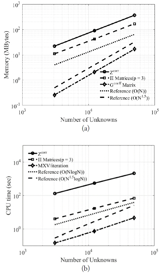
The numerical complexities versus the number of unknowns (p = 3) (a) Memory requirements. (b) The CPU time for the matrix-fill-in and matrix-vector products per iteration.
The accuracy of the IE-FFT algorithm for the MFIE formulation is addressed. The root mean square (RMS) error of the bistatic RCS is defined as
where θ and φ are the azimuth and elevation angles, RCSA (θ,φ) is the RCS value of the conventional MoM, the IE-FFT algorithm [9], and other numerical methods. First, we calculate the RMS error of the conventional MoM, relative to the Mie series solution versus the sampling segments per wavelength. The value of the error is the maximum error bound of the IE-FFT. For example, the RMS error of the bistatic RCS for a one-meter PEC sphere at a frequency of 600 MHz is 0.0108. Due to the hyper-singular integral of the MFIE formulation, the RMS error is much larger than that of the EFIE. The RMS errors of the IE-FFT, relative to the Mie series sampling segments per wavelength, are plotted in Fig. 7. The dashed line is the RMS error of the conventional MoM as a reference. The dash-dotted line with square markers and the solid line with circular markers represent the RMS error of the IE-FFT for the second- and third-order Lagrange polynomials, respectively. The RMS error of the second-order polynomials is converged with that of the conventional MoM with approximately 28 sampling segments. However, the RMS error of the third-order polynomials is converged with 19 elements. In this case, the RMS error for the MFIE is approximately 0.01. Some discrepancies are not the problem of the IE-FFT but that of the conventional MoM. The accuracy of the IE-FFT algorithm can be compared to that of the conventional MoM.
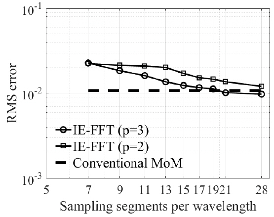
The RMS errors of the bistatic RCS calculations versus the sampling segments per wavelength (p = 2, 3).
V. Conclusion
The IE-FFT algorithm with MFIE formulation achieves O(N1.5) and O(N1.5logN) complexities for required memory and CPU time, respectively. Also, it is shown that the proposed algorithm is highly efficient without the help of a preconditioner. The IE-FFT algorithm with MFIE formulation provides a high convergence rate as well. For better accuracy, a new scheme of hyper-singular integration should be further considered.
References
Biography
Seung Mo Seo received the B.S. degree from Hongik University in 1998 and the M.S. and Ph.D. degrees from the Ohio State University in 2001 and 2006, respectively, all in electrical engineering. From 1999 to 2006, he was a Graduate Research Associate with the ElectroScience Laboratory (ESL) in the Department of Electrical and Computer Engineering, the Ohio State University, Columbus, where he focused on the development of fast integral equation methods. From 2007 to 2010, he was Senior Engineer at the Digital Media and Communication (DMC) R&D Center of Samsung Electronics, where he developed RF circuit and antenna designs and simulations. From 2011 to the present, he has worked as a Senior Researcher at the Agency for Defense Development. His current research interest is computational electromagnetics.